Wave Motion#
Background#
Overall goals and overview#
Understand wave propagation through a medium by investigating the relationship between wave frequency and wavelength using strings.
In this experiment, you will vary the frequency of the sine wave generator until you achieve standing waves. You will then measure wavelengths of vibrations at those frequencies for four cases of string/tension combinations: two different density strings at two different tensions. You will then determine the propagation velocity of the waves through the different mediums.
The general equation for the velocity of propagation of waves in a medium of continuously distributed stiffness and inertia is given by a formula of the form
In the case of transverse waves propagated along a flexible cord, the elasticity or stiffness factor is due to the tension, \(F_T\), in the cord; and the inertial factor is the linear density, \(\mu=m/L\), of the cord. Thus the velocity of propagation, \(v\), of a transverse wave is
The velocity can also be determined from (161) by establishing standing waves with a known frequency, \(f\). The wavelength, \(\lambda\), is directly measurable from the spacing of nodes, or points of zero displacement. (The wavelength is twice the distance between successive nodes.)
A standing wave is produced when two identical waves travel in opposite directions in the same medium. The two waves interfere with each other forming a pattern of vibration that is stationary along the direction of propagation.
For our case, a wave is generated at one end of a cord by a string vibrator that moves the cord up and down at a measurable frequency. This wave travels down the cord to the other end and reflects back towards the source. As the wave reflects back and forth, augmented by the string vibrator at one end, the oppositely traveling waves interfere to produce a ‘standing-wave’ pattern of vibration. It can be shown that certain points of this pattern never move. They are called nodes. Thus in order for a standing wave pattern to be produced on a cord that is effectively tied at both ends and cannot move, the pattern that is established must, at the very least, have nodes at each end.
It can also be shown that the spacing of nodes is \(\lambda\)/2. Since the propagation velocity is only a function of the physical properties of the cord, the wavelength can be adjusted by selecting the appropriate frequencies of vibration that satisfy the condition of ‘nodes at least at the ends’. Since the length of the cord must be such that nodes exist at each end, the length of the cord, tied at each end, must be an integral number of \(\lambda\)/2 and the allowable frequencies of vibration of the cord are integral multiples of each other. They are said to be harmonically related.
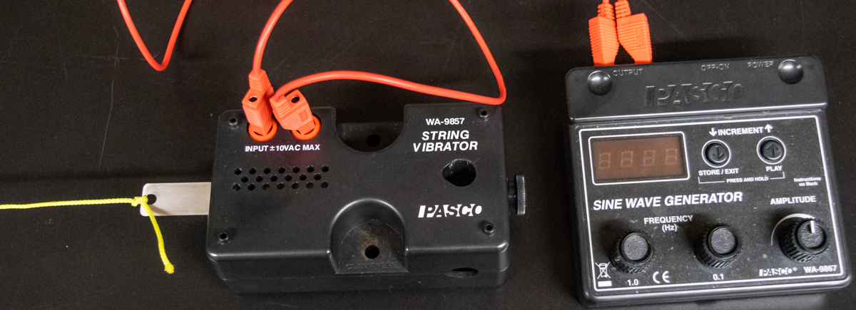
Fig. 132 Setup with sine wave generator and string vibrator.#
In this experiment, one end of a horizontal cord is attached to the string vibrator (see Figure 132) and the other end, after passing over a pulley, is attached to a hanging mass. We can adjust the amplitude and the frequency of the wave by adjusting the output of the sine wave generator, which powers the string vibrator. The tension is determined by the weight of the hanging mass. Therefore for a given tension and linear density, the frequency can be adjusted and measured for a standing wave condition. A measurement of node spacing establishes the wavelength. With the frequency and wavelength measured, the velocity can be determined from (161). From a measurement of the linear density of the cord and the tension in the cord, we can independently determine the velocity from (160). The two independently determined values of velocity of propagation can be compared.
Equipment#
Sine wave generator. 1 – 800 Hz with 0.1 Hz resolution. Coarse and fine adjustment knobs for 1 and 0.1 Hz increments. Amplitude knob to change how large the waves are (useful for keeping the string from hitting the table)
String vibrator
x2 banana-plug wires to connect sine wave generator to string vibrator
Meter sticks
Clamp to hold string vibrator to desk
2 strings of different linear densities (yellow and white, \(\sim 1 - 1.5\,\text{m}\) long)
Mass hanger with 200 g and 300 g disk masses
Low friction pulley to translate the weight of hanging mass to tension in the string
Experimental Procedure#
Measure the exact length of the cord by untying it completely and gently stretching it along a meter stick. Weigh it on a digital balance to the nearest thousandth of a gram and calculate its linear density (mass per unit length). Create a common data table with values for each cord including cord mass, cord length, and calculated cord linear density, \(\mu=m/L\). Include the accepted value of \(g\).
The four cases are the light cord and the heavy cord, each with 250 g and 350 g total mass using the mass hanger (remember to include the mass of the hanger):
Case I – white cord, 250 g
Case II – white cord, 350 g
Case III – yellow cord, 250 g
Case IV – yellow cord, 350 g
Create a common data table for each case with the hanging mass, the tension, the string linear density, and the calculated propagation velocity. Create a data table for the current case with columns for harmonic number (\(n = 1, 2, 3, 4, 5,\) and \(6\)) the measured wavelength \(\lambda_n\), the measured frequency \(f_n\), the ratio \(f_n/f_1\) of the frequency to the fundamental and the velocity \(v_n=\lambda_n f_n\).
Tie one end of the cord to the vibrating blade, run it over the pulley, and hang a total of 250 g from it using a mass hanger and the appropriate masses. Turn on the Sine Wave Generator and set the Amplitude knob about midway. Use the Coarse (1.0 Hz increments) and Fine (0.1 Hz increments) Frequency knobs of the Sine Wave Generator to adjust the vibrations so that the the cord vibrates in one segment. This first harmonic is achieved when the cord is vibrating at what is known as the fundamental frequency. Adjust the driving amplitude and frequency to obtain a large-amplitude wave that vibrates smoothly. Check vibration near the vibrating blade. Ideally, the point where the cord attaches should be a node, but you will find that the apparent position of the node is somewhere past where the cord attaches. Measure the distance between nodes and calculate the wavelength. For the first harmonic you need to estimate the position of the node near the blade. For higher harmonics, you can avoid the node near the blade and only use nodes at the pulley and along the string. What’s your estimated uncertainty in the length measurement; more or less accurate when measuring across single or multiple nodes?
Record the frequency. How much uncertainty is there in this value? Slightly vary the frequency and note how much you can increase or decrease the frequency before you see an effect.
Raise the frequency to resonate at the second harmonic. The cord should vibrate with a node at each end and one node in the center. Again measure the frequency and the distance between nodes.
Repeat the same measurements for the higher harmonics.
Determine the ratio of each frequency to the fundamental frequency, \(f_n/f_1\).
Compute the velocity \(v=f \lambda\) for each resonant frequency (trial); how do they compare to each other?
Calculate the average and standard deviation of the propagation velocity \(v\) and compare your avg. ± std. dev. with the theoretical velocity calculated from the tension and the linear density in (160).
Plot wavelength \(\lambda\) vs. the inverse of the frequency \(1/f\) and use the slope to determine the propagation velocity. Also consider the uncertainty in the slope. Does your plot-derived propagation velocity agree with the theoretical velocity as calculated in the previous step? Your plot will be represented by the reorganization of (161):
CONSIDER: How do you expect tensions and linear densities to affect the wave propagation?
Increase the hanging mass to 350 grams and repeat the above procedure for Case II.
Using a cord with a different density repeat steps 4 to 13 for Case III and IV.
Post-Lab Submission — Interpretation of Results#
Make sure to submit your finalized data sheet with summarized data and cleaned-up plots (Excel sheet)
Paragraph of your results +/- uncertainties from your data. Make sure to include discussion of the following:
For each of the four cases, give the theoretical velocity from (160), the average and standard deviation of your results using (161), and your value from the slope in Step 11.
Do the velocities of propagation found by two methods (average values from each case, plot fitting) agree with the expected values? Of the two methods, which would you trust more and why; was there a physical or statistical reason?
How is the velocity of propagation dependent on the tension in the string and density of the cord; when the experiment was done with a lighter weight cord, why would the string vibrator have to be run faster for each measurement condition?
Paragraph of your errors and estimated measurement uncertainties. Be quantitative. Make sure to include discussion of the following:
Where might systematic (affecting accuracy) and/or random (affecting precision) errors be coming from?
What are your measured uncertainties, and, based on these uncertainties, how do your final results change? I.e. do your different measurement and slope uncertainties make your final results larger or smaller?
Change different variables by your best estimation of measurement uncertainties in your Excel sheet; what variables affect the accuracy of your final results the most?
If larger or small, are they more or less accurate to expected values?
How could you improve your random errors or make your measurements more accurate?
Were your systematic errors significant; how could this be improved if you were to re-run this experiment?
Reflect on this week’s lab; what did you learn?
The Whiteboard#
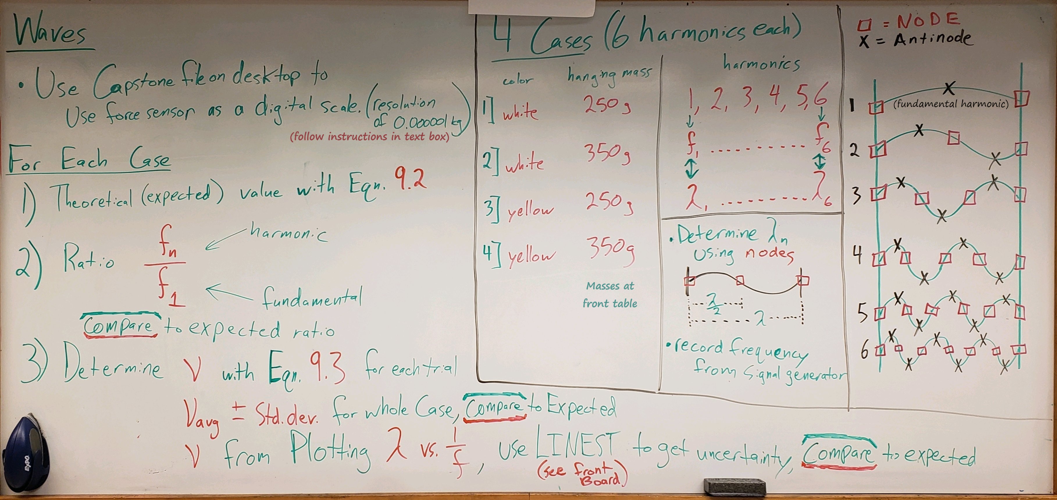
Fig. 133 Overview.#
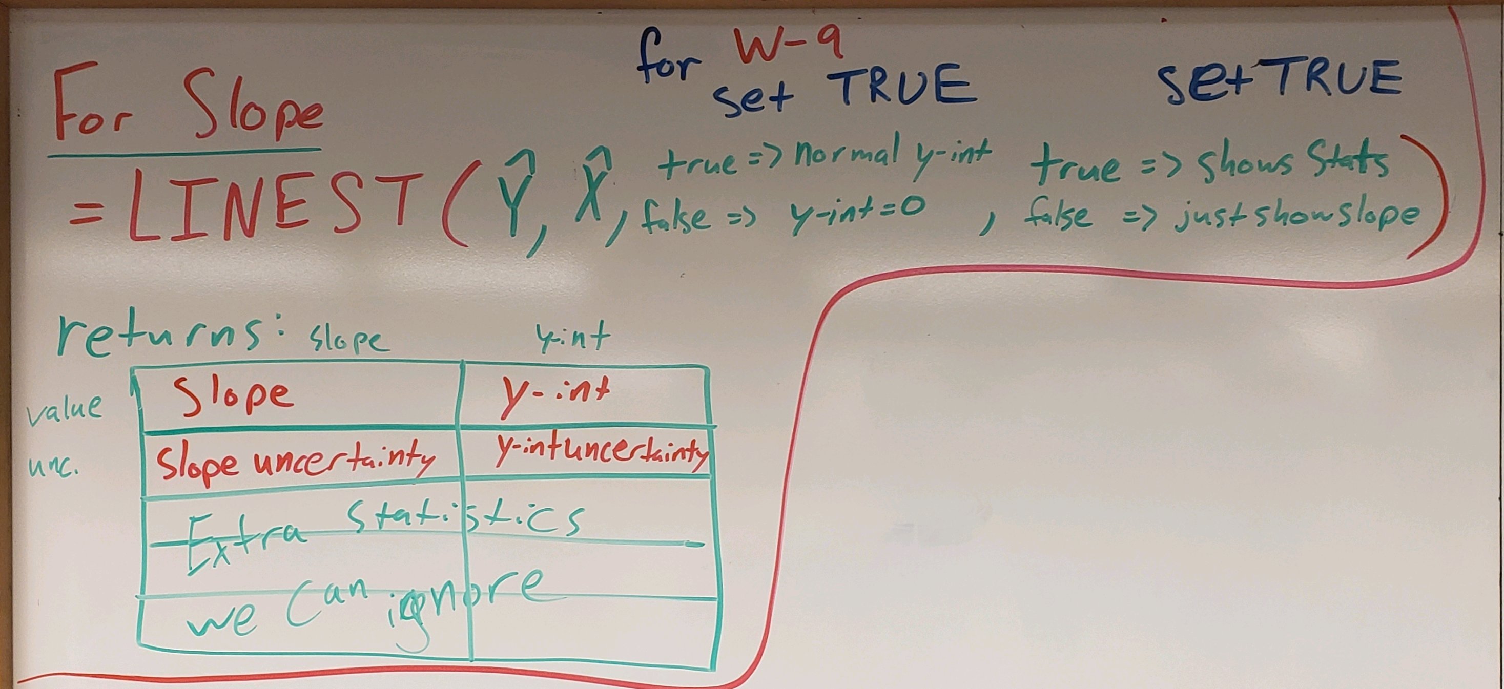
Fig. 134 LINEST() function.#