Acceleration due to Gravity, g, with Glider on Tilted Air Track#
OVERALL GOALS
Use an frictionless airtrack to:
Measure acceleration due to gravity.
Background#
By measuring the acceleration of a mass moving under the influence of just the gravitational attraction of the earth, namely its weight, we can determine the acceleration due to gravity, usually denoted by \(g\). The mass will be allowed to accelerate down a presumed frictionless, inclined plane. Measurement of the acceleration along the plane is directly related to the acceleration due to gravity by a simple trigonometric relationship. The use of the plane permits the convenient measurement of a small, measurable fraction of the acceleration due to gravity. This of course is in lieu of the much more difficult measurement of a vertically falling mass.
Near the surface of the earth, the attractive force of the earth on a mass can be considered a constant over a reasonable range of elevation. This force is commonly called the weight of the object and, from Newton’s Second Law, the weight is the mass \(m\) times the acceleration due to gravity \(g\). Using Fig. 26 and the derivation following, we can see that the value of \(g\) can be easily determined by a few simple measurements.
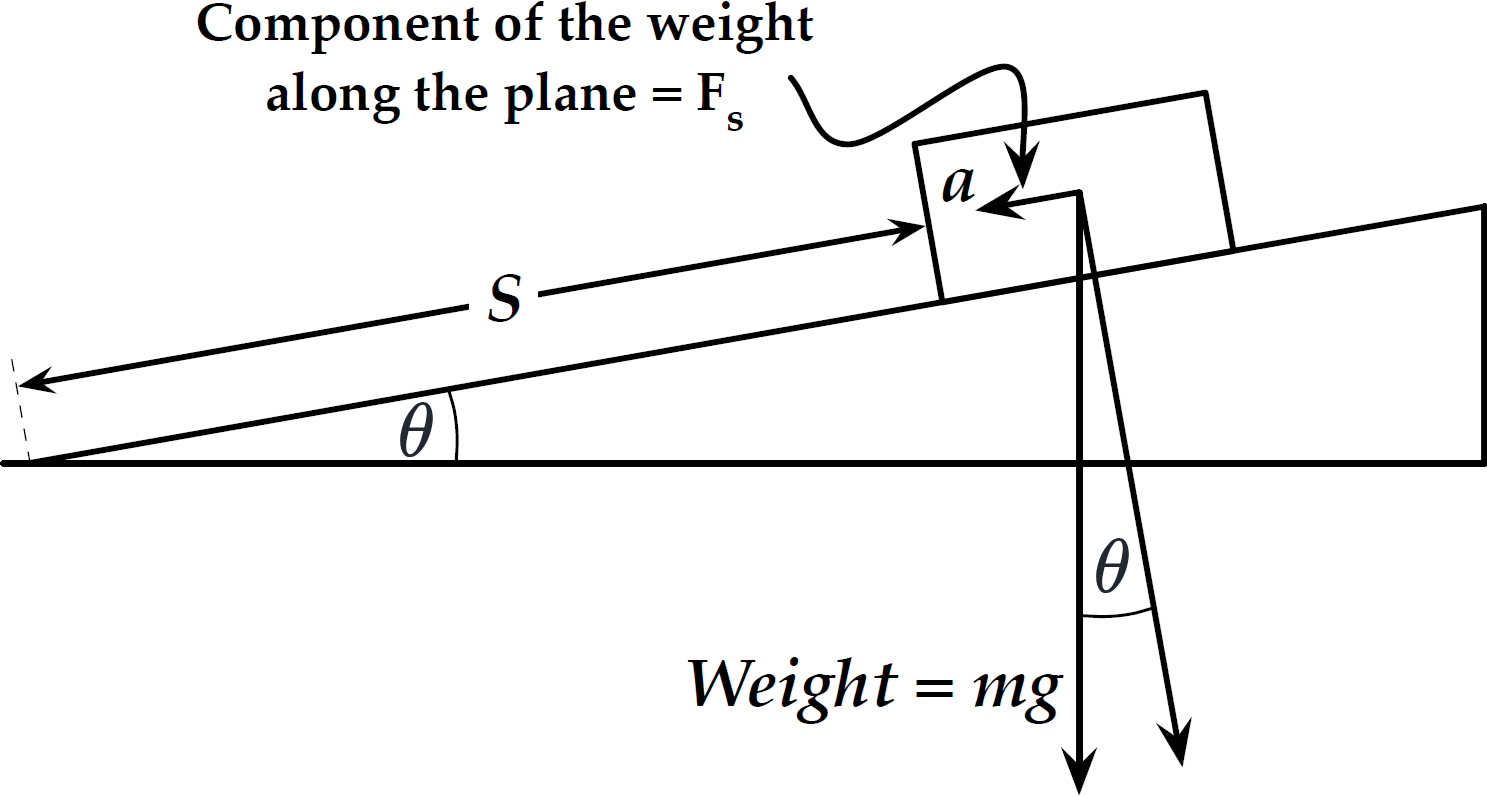
Fig. 26 Force diagram based on the angle of the tilted air track.#
The displacement along the track is \(S\), the component of the weight along the track is \(F_s\), and the component of acceleration \(a_s\) along the track is
If the mass is released from rest near the top of the inclined air track and allowed to accelerate down the air track with a magnitude \(a_s\), then by measuring the transit time down the track over a measurable distance \(S\), we can determine the value of \(g\).
Since the acceleration \(a_s\) is constant as gravity itself is constant, the displacement \(S\) as a function of time \(t\) is:
Solving for \(g\), we obtain
where, based on our schematic of the experimental setup in Fig. 27, we see \(\sin(\theta) = \frac{H}{D}\). Making this substitution for the \(\sin(\theta)\), we have the value of \(g\) in terms of easily measurable quantities, namely
where \(H\) is the vertical rise in the horizontal distance \(D\). \(D\) is the distance between the legs of the air track, and \(t\) is the transit time of the mass, starting from zero velocity and accelerating down the plane a distance \(S\) along the plane.
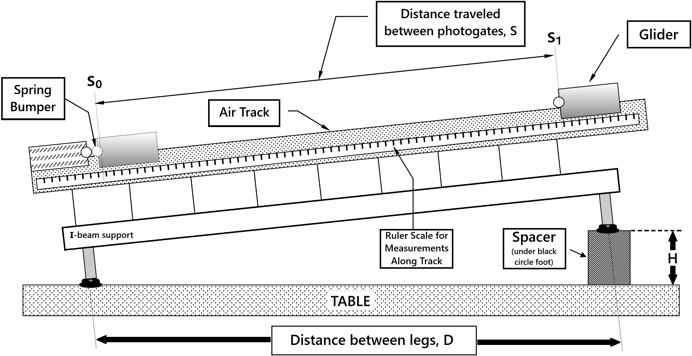
Fig. 27 Experimental Setup.#
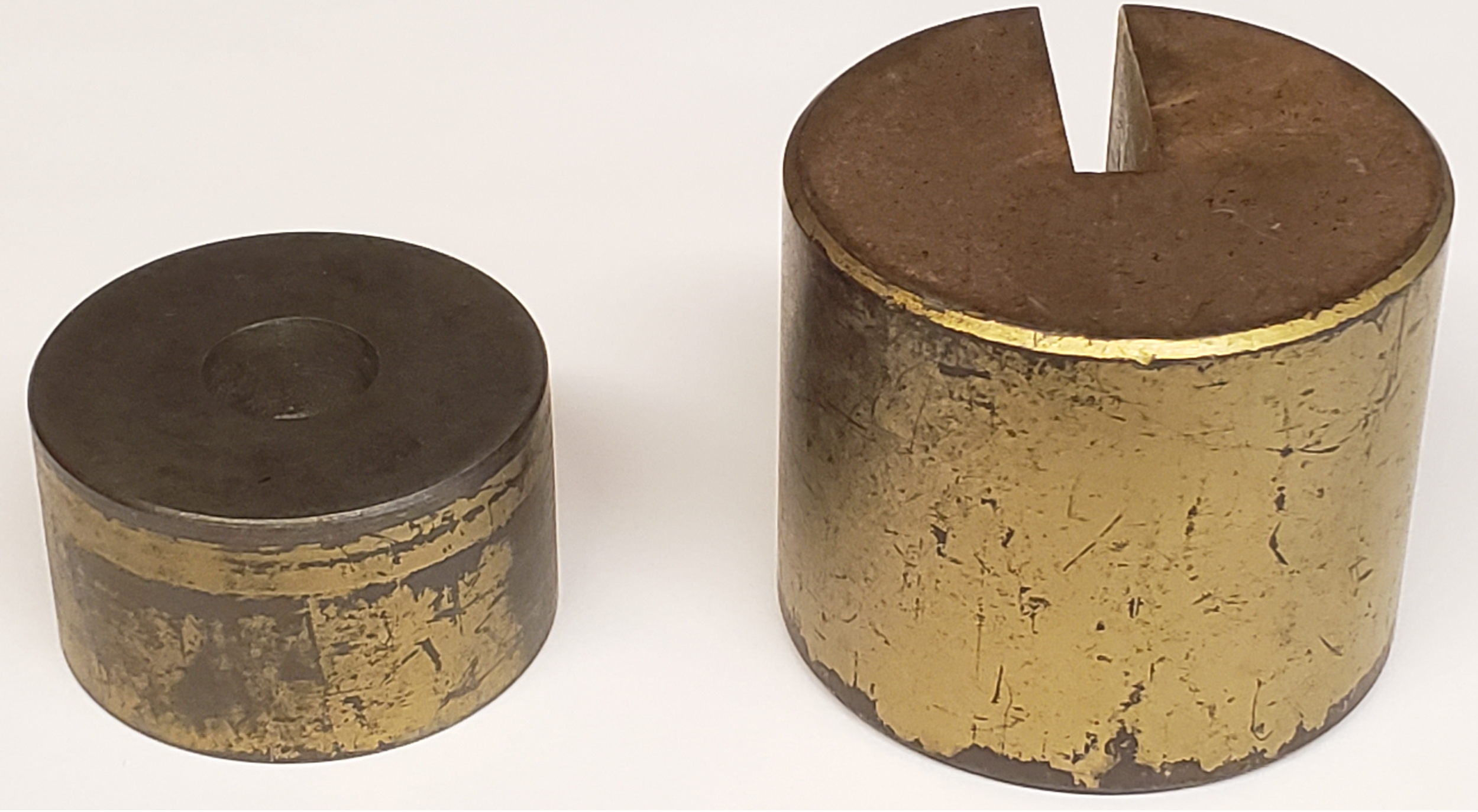
Fig. 28 Example of small and large spacers used to incline the air track. Remember to put the black plastic footer (not shown) on top of the spacers.#
Experimental Procedure#
Procedure Preview#
OVERVIEW
Experimentally determine the acceleration due to gravity \(g\) by using a slightly tilted airtrack.
Investigate how \(g\) is affected by the mass of an object and angle of the track (i.e. initial height of that object).
Conduct 4 cases based on 2 glider sizes and 2 initial heights.
Each case will have a total of 6 trials:
Groups of 2 students, each student will release the glider for 3 trials
Groups of 3 students, each student will release the glider for 2 trials
Compare the experimental results to the expected value of \(g\) at Fairfield, CT, of \(9.803\,\text{m/s}^2\).
Notes & Assumptions
The presumed frictionless inclined plane will be an air track.
The mass will be a glider, which floats on the air track.
Placing a spacer (essentially a big slotted mass, see Fig. 28) of height \(H\) under the leg at one end of the track, which is a distance \(D\) from the leg(s) at the opposite end, will incline the track.
Time measured by PASCO photogates (stated precision of 0.0001 seconds). Using PASCO’s data logging and visualization software, Capstone, installed on the lab computers. The relevant Capstone file will be on the desktop. Please DO NOT save when you are done, just exit without saving, thanks.
Preliminary Setup#
Do not put a glider on the track without air flowing. If the air supply is not yet on, please remind the instructor.
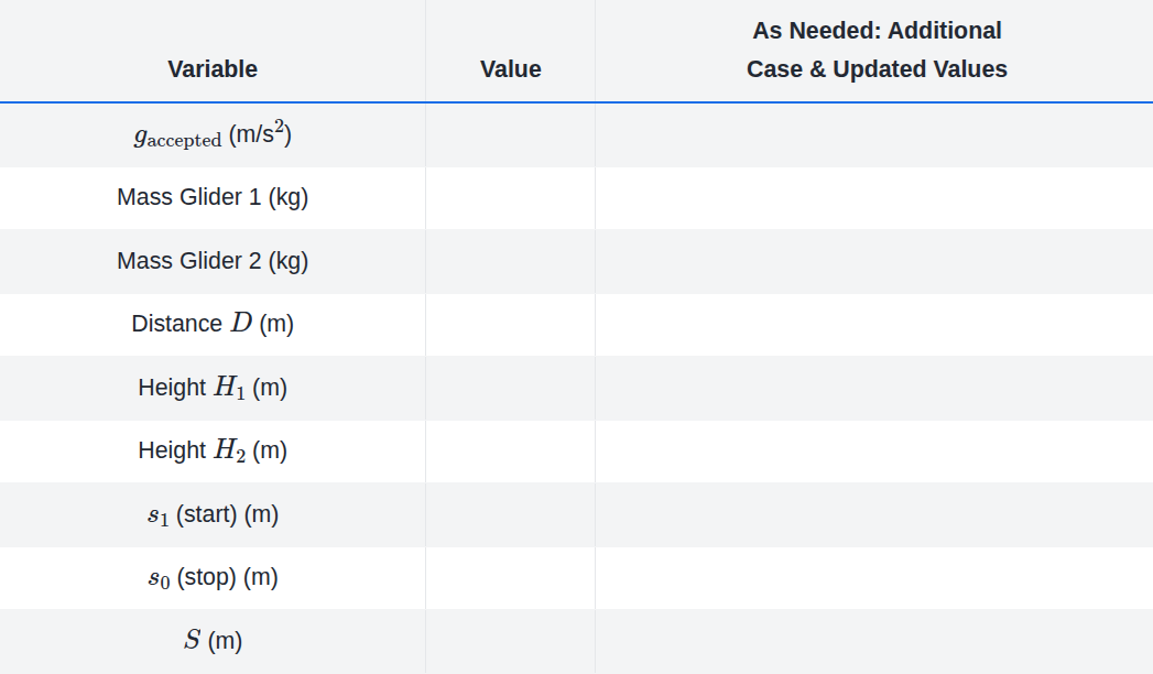
Create a common data table including (e.g. Example Common Data Table):
accepted value of \(g\) of \(9.803\,\text{m/s}^2\) for Fairfield, CT
the masses of each of the gliders in kg
the distance \(D\) between the legs of the air track in meter (m)
the heights \(H\) of the two spacers (big slotted masses) in m
\(s_1\): starting point at the top
\(s_0\): stopping point at the bottom
\(S\): distance between the photogates that the glider travels along the track
Measure and record the mass of both the big and small glider with the triple-beam-balance.
Calibration
Reminder: ensure the balance is zeroed before measurements. You can use the adjustment knob on the left side under the silver weighing platform to ensure the pointers at the right end are aligned.
Level the airtrack. Without the spacer present and the air track resting directly on the tabletop (with the black circle feet), place one of the gliders on the track (somewhere between the photogates, center) and note any preferential drift of the glider. Adjust the height of the single leg (screw clockwise in or counter-clockwise out) until the air track is level, as indicated by no preferential drift. Check both orientations of the glider on the track to check if the car is asymmetric and has a significant preferential drift on an otherwise level track. If this occurs, make sure to note that for your discussion purposes. <!—request the use of another glider and we can provide you a different one.—>
Drift
There will inevitably be some drift as these airtracks are not perfect, but as a general rule of thumb, if it takes more than \(\sim 10\) seconds to drift just 5 cm, you should be pretty good.
Measure and record the distance \(D\). This is the center-to-center distance between the legs. 1 m and 2 m long meter sticks are available for this measurement, with additional meter sticks at the front wall of the room.
Measure and record the heights, \(H\), of each of the two spacers (big slotted masses) with the provided Vernier caliper. If you need a refresher on using Vernier calipers, see Reading the Vernier scale.
Take a look at the gliders and determine a convenient point on the glider to use with the scale (\(\sim2.5\) meter ruler) attached on the side of air track. It doesn’t matter what point on the glider you choose, only that you be consistent and use the same point for all determinations of distance along the track \(S\) for that glider. A convenient point is the lower front or rear corner of the glider since it is a clear point on the glider that will overlap or be quite close to the length scale on the track itself (see Fig. 29).
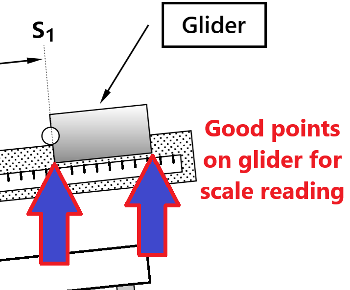
Fig. 29 Suggested points on glider to read position on airtrack scale.#
Determine and record the bottom photogate position \(s_0\) at the bottom end of the track. Place the glider near the bottom of the track. Move it slowly as you approach the bottom photogate. Stop the glider at the exact location when the photogate’s red light comes on. Move the glider back and forth to confirm your scale reading. See Demo Video: Photogate Positions for example method.
Demo Video: Photogate Positions#
Similarly, determine and record the starting photogate position \(s_1\) at the top end of the track. Place the glider near the top of the track. Move it slowly as you approach the top photogate. Stop the glider at the exact location when the photogate’s red light comes on. Move the glider back and forth to confirm your scale reading. Ensure your scale reading on the track was based on the same location of the glider as for your \(s_0\) reading (i.e. Fig. 29).
Accurate Photogate Positions
Be careful not to bump the photogates, as that could change their positions and lead to inaccurate distances. Check during each case; if need be, expand your common data table with additional \(s_0\) and \(s_1\) positions.
Four cases will be performed as listed in Table 5. For each of the four cases, perform the following steps listed in Experimental Data Collection and record the data appropriately in your spreadsheet.
Table 5 Four experimental cases with spacers and gliders# Case
Spacer Size
Glider Size
1
BIG
small
2
BIG
BIG
3
small
small
4
small
BIG
Reminder, Run First Case Fully
Reminder, run your first case completely before moving on to additional cases. Don’t just take all of your data without checking your methodology. If you have some error in your experimental method or in your calculations, you can correct it before completing all the other cases and finding out you have to completely redo the whole lab. The data tables for additional cases can be created by copying the first case after you are confident in and can explain your results from the first case.
Experimental Data Collection#
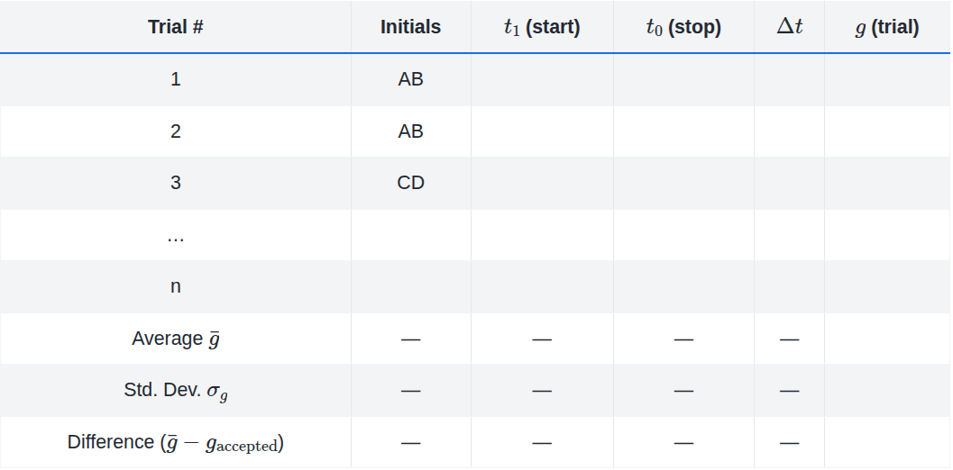
For each of the four cases, create a Data table with enough rows for the number of trials you are doing, and columns for each of the variables you will be measuring or deriving (e.g. Example Case Data Table):
Trial number
Lab member’s initials
\(t_1\): start time at the top
\(t_0\): stop time at the bottom
\(\Delta t\): time of travel between the photogates
\(g\): experimentally determined value of \(g\) for each trial
\(\bar{g}\): average value of \(g\) from the trials of each individual case
\(\sigma_g\): standard deviation of \(g\) from the trials of each individual case
difference (magnitude, not percent) between the average value of \(g\) and the accepted value for each case
Ensure \(s_1\) and \(s_0\) haven’t changed.
Raise the single leg side of the track by placing the case-relevant spacer under the black foot as seen in Fig. 27.
Before you take the recorded data in the next steps, take some practice runs. Your subsequent data will be much improved by your training! Press record in Capstone to start the timer.
Capstone Timer
The timer shown is coded in Capstone; once you press record, it will take a few seconds for the timer to start, wait until you confirm the timer is ready before releasing the glider.
Capstone will display the time whenever a photogate beam is broken; the time shown is the time at the higher (start) photogate \(t_1\) as well as the time at the lower (end) photogate \(t_0\). To determine the total transit time \(\Delta t\), take the difference of the start and end times.
Additional notes on the timer are in the Capstone file itself, please read.
For each of the 6 trials per case, release the glider from rest at the \(s_1\) position. Measure and record the start time \(t_1\) and end time \(t_0\) to determine transit time \(\Delta t\) from the release at the top to bottom of the airtrack. Calculate the value of \(g\). To do so:
a. Position the glider so it is blocking the top photogate and the red light is on. Use the red glider-release mechanism to hold the glider in place. Shift the mechanism up or down the track as necessary to hold the glider just before the photogate beam such that the red light on the photogate just goes out.
b. Check the Capstone timer is ready, then release the glider by quickly flipping the glider release bar to minimize any additional push or pull on the glider to ensure its initial velocity is zero. See example in Demo Video: Glider Release.
Demo Video: Glider Release
Demonstration of glider release to minimize initial velocity. c. Record the relevant \(t_1\) and \(t_0\) values in your spreadsheet. Calculate \(\Delta t\), and \(g\) for this trial using (35).
d. Repeat for each trial of this case. Reminder, you do not need to turn off the timer, you just need the relevant times as you will be using the time difference.
Reminder: Take turns
Groups of 2 students, each student will release the glider for 3 trials
Groups of 3 students, each student will release the glider for 2 trials
From the 6 trials of this case:
Calculate \(\bar{g}\), the average of the measured \(g\)
Calculate \(\sigma_g\), the standard deviation of the measured \(g\)
Calculate the difference between your average \(g\) and the accepted value of \(g\) (e.g. \(\bar{g} - g_{\text{accepted}}\))
Repeat the previous steps for the next case, only after you’ve completed all calculations.
Continue to additional case?
If you are satisfied your calculations are complete and results seem reasonable (feel free to check with your professor), it is at this point that you may continue to the next case.
Combined Results Across All Trials#
Create an Overall data table summarizing all 24 trials across all 4 cases (e.g. Example Overall Data Table):
Calculate \(\bar{g}_{\text{allTrials}}\), the average of the measured \(g\)
Calculate \(\sigma_{g\text{,allTrials}}\), the standard deviation of the measured \(g\)
Calculate the difference between your average \(g\) and the accepted value of \(g\) (e.g. \(\bar{g}_{\text{allTrials}} - g_{\text{accepted}}\))
Post-Lab Submission — Interpretation of Results#
Make sure to submit your finalized data table (Excel sheet)
In a paragraph, summarize the results you have determined in each case, i.e. \(\bar{g}\pm\sigma_g\)… and answer the following questions (longer does not mean better):
If you release the glider with an initial velocity up or down the slope, what would you expect to happen to your derived values of \(g\)?
Suppose there is a frictional force slowing the glider as it moves along the track. How would this affect the determined value of \(g\)? Would your result support or not support the hypothesis of that there is significant friction along the track?
Assume the track is not level at the beginning of the experiment. Further, assume that what you thought to be a level track was in fact slightly tipped in the same direction as your deliberate tipping via the spacers during the experiment. How would this affect the determined value of \(g\)? Would your result support or not support the hypothesis of the track not being level?
In a paragraph, summarize your error analysis. Be qualitative not only quantitative.
What are sources of uncertainty (initial v, friction, etc.)?
What was the precision of the instrumentation (e.g. caliper, time, distance, etc.)?
Compare your results (\(g\) from each of the four cases and one from all 24 trials) to the accepted value. How do the standard deviations compare to the difference between your values of \(g\) and the accepted value of \(g\)?
I.e. while treating the standard deviations of your measurements as your measurement uncertainties, do your values of \(g\) for each case, as well as the overall average \(g\), plus or minus the standard deviations overlap (and agree) with the accepted value of \(g\)?
What might cause your results to disagree the most?
The Whiteboard#
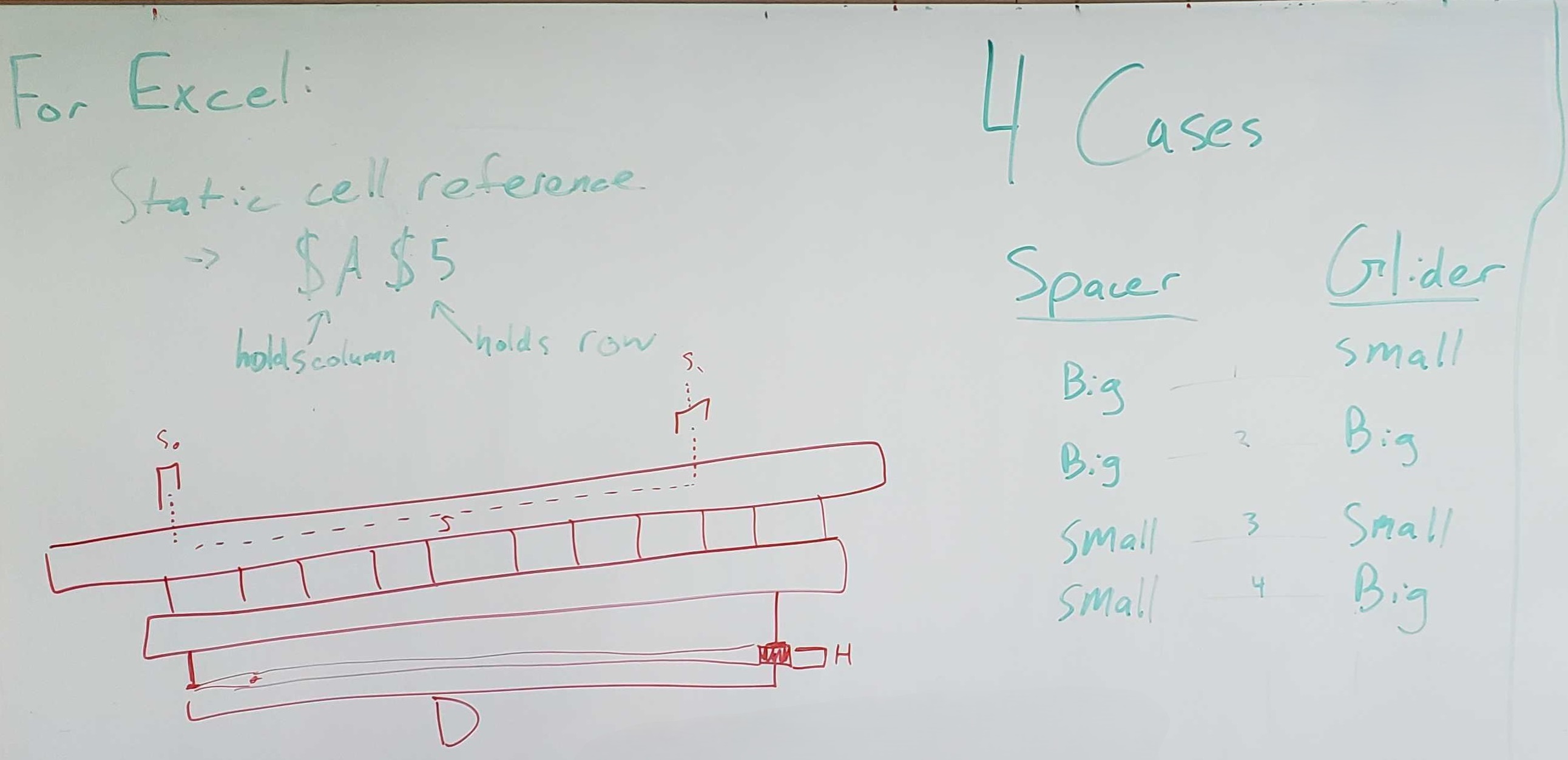
Example data tables are shown below to assist you in building your spreadsheet for this lab. Additionally the original whiteboard summary is at the end of this section.
Example Common Data Table#
Example Case Data Table#
Example Overall Data Table#

Original Whiteboard Info#