1146L-ONLY | Light – Geometric Optics and Imaging#
Danger
⚠️ LASERS IN USE TODAY ⚠️
DO NOT SHINE THE LASER INTO ANYONE’S EYES
YOU AND OTHERS CAN GO BLIND
Background – Part I – Multiple Slit Diffraction#
Overall goals and overview#
Investigate diffraction of light and its relation to multiple-slit spacings and light wavelength with a monochromatic laser.
Investigate reflected light diffraction and its relationship to size of the reflective object’s topography, again with a monochromatic laser.
Investigate light refraction through lenses, both unfiltered and chromatically or spherically filtered by determining focal lengths with image and object distances.
In today’s lab, you will complete three experiments:
Experiment 1: Shine a laser through multiple slits of known spacing, creating a diffraction pattern on a far wall. Tape a piece of paper centered on the pattern, trace the pattern, then measure the spacing between the dots. Determine the wavelength and compare to the actual value of the laser.
Experiment 2: Shine a laser on a music CD to create a reflected diffraction pattern. Using the spacing of the diffraction pattern and wavelength determined in Experiment 1, determine the spacing between the physical tracks (pits) indented in the plastic of the CD. Compare to the known value given in the procedure. Consider how the diffraction spacing relates to the topography of the CD.
Experiment 3: Determine focal lengths of the lens first unfiltered at various distances, then chromatic filtering through red and blue filters, then spherical aberration near center and edge of the lens; consider the physical reasoning for longer or shorter focal lengths depending on differences in the filtering or refracting of the light source. Plot image vs. object distance pairs for the unfiltered distances and investigate the convergence point; compare that value to your average of focal lengths from the unfiltered portion of this experiment.
Multiple slit diffraction will be used first to find the wavelength of a laser light source. Having determined the wavelength of the laser light, that combined with the reflected diffraction pattern will be used to determine the spacing between the tracks of a standard music CD (compact disc).
To understand diffraction, we will consider the interference of various parts of a wavefront as they emerge from a transmission diffraction grating. The transmission grating is much like the openings formed by partially open window blinds. The diffractive effects result from the interference of the various portions of the same wavefront as they are formed by passing the wavefront through the diffraction grating.
The number of slits that are actually used in the experiment is very large. To quickly understand diffraction from multiple slits, we will consider the pattern of constructive interference of the portions of the wavefront that emerge from two, narrow slits, spaced a distance \(d\) apart as illustrated in Figure 135.
Fig. 135 Two-Slit Wavefronts#
The analysis of the resulting diffraction pattern after the light passes through the slits rests on two fundamental principles. The first, Huygen’s principle, states that each portion of a wavefront can be considered a separate radiating source. The second is linear superposition; that is, the total field vector at any given position is the vector sum of the individual field vectors simultaneously present.
The portion of the wavefronts that are present in the slits are considered Huygen sources of radiating spherical wavelets. The wavelets then interfere with each other to form new wavefronts. (If a plane wave were radiating unimpeded in free space, each of these wavelets would interfere to form additional plane waves propagating in the same direction as the original wavefront.) However, when portions of a wave-front are deleted as they are here, the interference will form a diffraction pattern that is very different from the plane wave that would have been formed (see example in Figure 136).
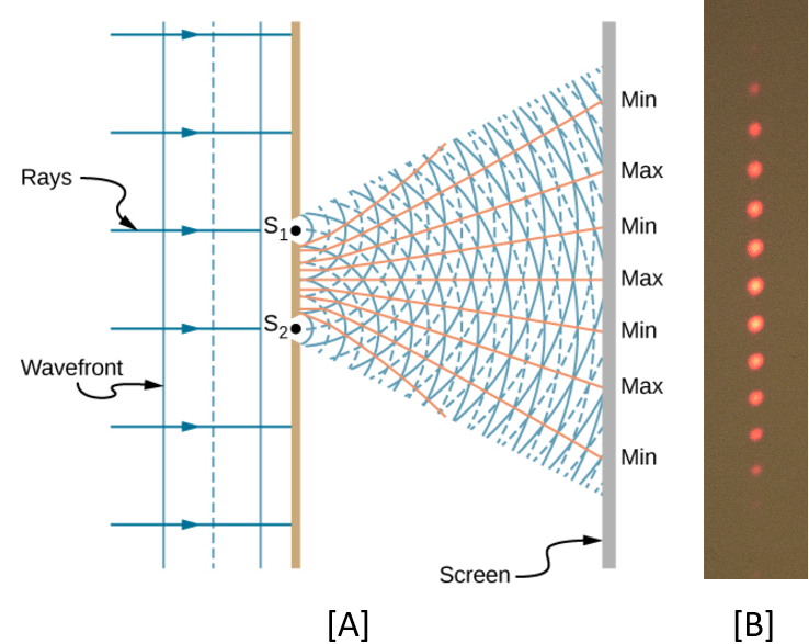
Fig. 136 Double Slit Diffraction. (A) Light spreads out (diffracts) from each slit, because the slits are narrow. These waves overlap and interfere constructively (bright spots) and destructively (dark regions). We can only see this if the light falls onto a screen and is scattered into our eyes. (B) When light that has passed through double slits falls on a screen, we see a pattern such as this.#
Consider the schematic in Figure 137; when the path length difference is equal to an integral number of wavelengths of the light, then the wavelets from each of the slits will constructively interfere and produce a bright spot. Notice that this condition occurs at angles when
where \(n\) is an integer (\(\pm\)) and \(\lambda\) is the wavelength of the light.
Thus we can expect to see bright spots on the wall/paper/board, when the angle from the initial direction of the laser beam satisfies the above criterion. For the small angles we are dealing with here, the distance from the initial bright spot, when \(n\) = 0, and therefore \(\theta\) = 0, to each of the diffracted spots is given by
where \(X\) is the distance to the screen, and \(n\) is the order number.
Combining these two equations
For small angles, \(\sin\theta_{n} \sim \theta_{n}\) (in radians). For the small angles we are dealing with here, the distances \(y\) are very small with respect to \(X\). Under these conditions, you can measure the distance between neighboring spots and then average all of these measurements to get a reasonably good number to use for \(\Delta y\). From (165), \(\Delta y = X \lambda / d\), or
The slit spacing \(d\) is given, you determine laser wavelength, and you can compare your results with the known wavelength of the HeNe (Helium Neon) laser you are using.
Fig. 137 Double Slit Diffraction#
Equipment#
Experiment I
The setup will appear in similar form to that seen in Figure 138 with laser pointed towards the diffraction grating which creates the diffraction pattern as seen earlier in Figure 136 right.
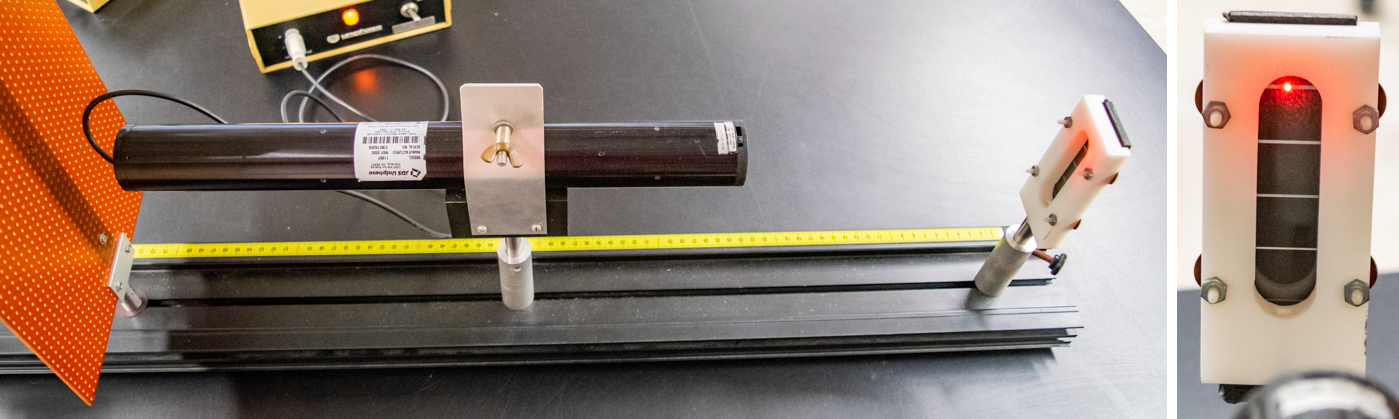
Fig. 138 Left) Laser mounted on black optics track pointed towards the diffraction grating as seen on the right.#
Diffraction grating with multiple slits of spacing \(d=0.20\,\text{mm}\)
Red HeNe laser with known value \(\lambda_{\text{HeNe}}=632.8\,\text{nm}\) and power source
Black optics track to mount everything
30 m long metric tape measure
White paper and tape
Experiment II, discussed further after experiment I.
Music CD with \(\sim 1.6 \times 10^{-6}\,\text{m}\) track spacing (see close-up example in Figure 139 left)
Red HeNe laser with known value \(\lambda_{\text{HeNe}}=632.8\,\text{nm}\) and power source
Black optics track to mount everything
Metric ruler vertically mounted with hole to allow laser to pass through
Experiment III, discussed further after experiment II.
Black optics track to mount everything
Light box with image on it (position of image noted by indented metal aligned with the ruler on the optics track) with power brick
Convex lens in lens holder (position of the lens in the holder is noted by a small plastic protrusion on the side of the holder to be lined up with the ruler on the optics track)
Red and blue filter – attaches to light box
Disk and annulus mask filters – attached to lens holder
White viewing screen (movable along the optics track)
\pagebreak
Experimental Procedure – Part I: Multiple Slit Diffraction Grating#
Danger
DO NOT SHINE THE LASER INTO ANYONE’S EYES
YOU AND OTHERS CAN GO BLIND
Turn on the laser and allow the beam to pass through the diffraction grating and form the diffraction pattern on the far wall. Tape a white sheet of paper on the wall at the position of the pattern. You should see a center bright spot with a series of evenly spaced diffraction spots above and below the center bright spot.
WHILE BEING CAREFUL NOT TO LOOK BACK INTO THE LASER, mark the location of each spot on the paper by carefully circling each spot on the paper.
Using the steel metric tape measure, measure the distance from the diffraction grating to the paper screen on the blackboard.
Remove the paper. Measure and record in a data table the coordinate of the center of each spot relative to the bottom edge of the paper (to have a consistent spot to measure from). Calculate and record in the data table the center to center distances between each spot and its nearest-neighbor spot by subtracting their coordinates. Calculate and record the average and standard deviation of these distances. As you can see from (164), the spacing should not be exactly the same. However, for the very small angles and range of angles we have here, they can be considered evenly spaced. This is of course the small angle approximation of the sine function.
Calculate the wavelength of the laser using (166) and compare it to the known value \(\lambda_{\text{HeNe}}=632.8\,\text{nm}\). The diffraction grating spacing is \(d=0.20\,\text{mm}\), \(200\,\mu\text{m}\), many times larger than the spacings of the CD tracks you will see in Part II.
Background – Part II – Reflected Diffraction Pattern#
For the second part of the diffraction experiment, we will use the now known wavelength of the light source to measure the spacing of an unknown array of slits. The unknown slits are the tracks of a CD (compact disc) with a zoomed in example shown in Figure 139.
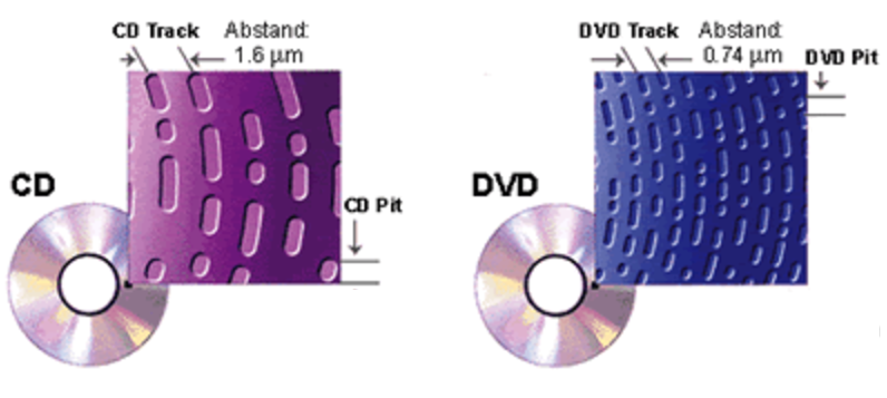
Fig. 139 Topography of a CD ROM. Lower capacity music CD on left, higher capacity DVD on right where the tracks are more closely packed together.#
Regarding a CD, before data is written to it, you would have just a flat surface. During manufacturing, for data to be written to the CD, a long, spiral track containing all the data (songs in the case of a music CD) is stamped into the plastic. This process creates little divots, called pits, into the plastic substrate; that surface is later metalized with aluminum to create a shiny, reflective surface. The spiral track is made to be a consistently spaced, spiral line of pits and flat surfaces that are \(\sim 1.6 \times 10^{-6}\,\text{m}\) or \(1.6\,\mu\text{m}\) apart (see Figure 139). To a laser, these pits act like slit-shaped mirrors that can reflect the laser light back at different angles, effectively creating the sources a new spherical wavelets. The subsequent reflected wavelets will interfere either constructively or deconstructively and create a reflected diffraction pattern whose characteristics depend on the wavelength of the laser and spacing the of CD tracks. Thus the analysis is the same as the transmission slits we used in part I, except we will reflect the laser beam from the CD rather than transmit it through as we did before. Because the spacing of the tracks of the CD are very small, the diffraction angles are large and small angle approximations cannot be used.
Fig. 140 Reflection Diffraction of CD ROM#
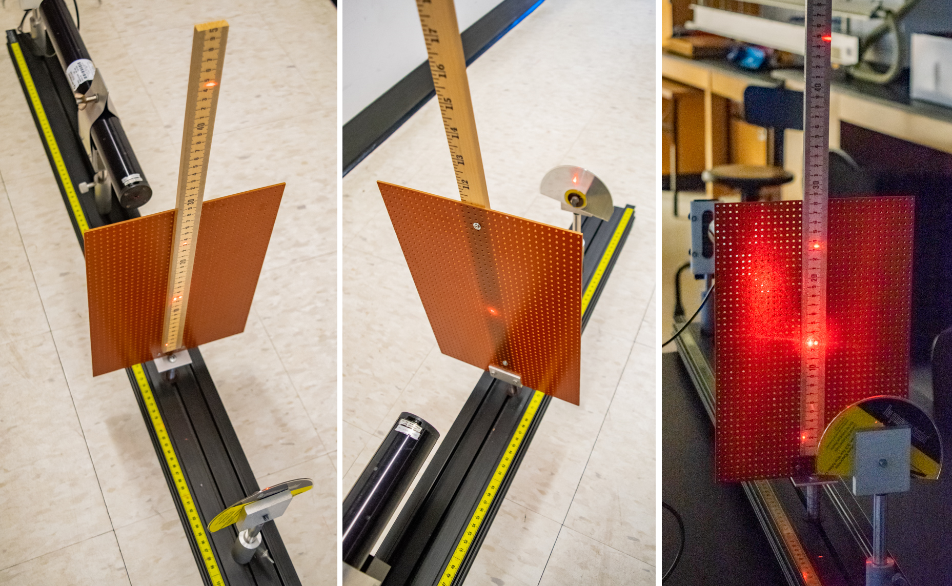
Fig. 141 Left) Laser mounted on black optics track pointed towards the CD. Center) Laser light passes through the ruler and reflects off the CD to create the diffraction pattern in (right).#
The experiment is configured as illustrated in Figure 140 and an example of the setup is in Figure 141.
The spacing of the tracks of a CD are so small that you will see only the first order diffraction spots, i.e. \(n = \pm 1\). With the large angle \(\Theta\) expected, the distance \(X\) can be about 30 cm and a standard sheet of graph paper can be used for the paper screen. From your measurements of \(X\) and \(\Delta y\), determine the diffraction angle \(\Theta\) from the tangent relation. Using (164), we can solve for the track spacing, \(d\), as
Experimental Procedure – Part II: Reflection Diffraction Grating#
Danger
DO NOT SHINE THE LASER INTO ANYONE’S EYES
YOU AND OTHERS CAN GO BLIND
Turn off the laser before moving it. Set up the laser and CD ROM as shown schematically in Figure 140. Turn on the laser and adjust the apparatus so the bright, center spot is directly back towards the laser. You should see the first order diffraction spots, one above and one below the center bright spot and a second order diffraction spot above the center spot.
Using the scale, measure and record the distances \(\Delta y_{1}\), \(\Delta y_{-1}\) and \(\Delta y_{2}\).
Average the \(\Delta y_{1}\) and \(\Delta y_{-1}\) and record the value.
Calculate the track spacing for each first-order diffraction spot and average the two determinations. Compare your calculated track spacing with the microscopically determined track spacing \(1.6 \times 10^{-6}\,\text{m}\).
Calculate the angle of the second-order diffraction spot using (163). Compare the height \(\Delta y_{2}\) of the second-order diffraction spot with the calculated height from (164). Notice that you cannot use the small angle approximation here.
\section{Background~\textendash~Part III~\textendash~Geometric Optics & Single Element Imaging}
Under many circumstances, the behavior of light can be analyzed by assuming that light travels in straight-line paths called light rays. Light rays are a representation of what is actually a very narrow beam of light. Using this representation of light, the behavior of many optical elements such as lenses and mirrors, and optical instruments such as telescopes, microscopes and projectors can be analyzed. The use of the ray model draws heavily on geometry, and is called geometric optics.
In addition to using the ray model of light, the lens that will be used will be analyzed under the thin lens approximation. This approximation will assume that the thickness of the lens is very small compared with the focal length. The result of this assumption is that the bending of the rays as they pass through the lens is considered to have occurred at a plane surface through the mid-line of the lens, perpendicular to the principal axis. Actually, the bending (the refraction) occurs at both the entrance and exit surfaces separated by a finite distance.
In this experiment, the behavior of a simple lens will be investigated with the setup (example in Fig. 142).
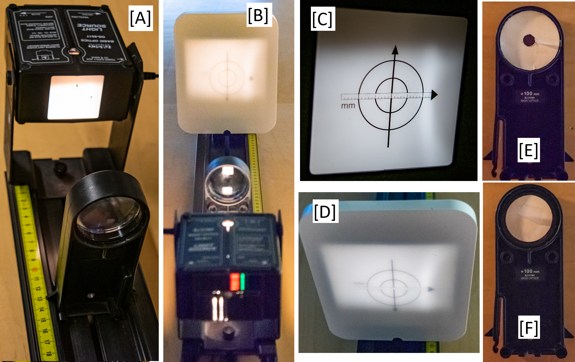
Fig. 142 A) Light box and lens mounted on optics track. B) Lightpath through lens onto the white screen. C) Image on the light box. D) Refracted image through the lens on the white screen. E) Annulus filter to allow light through center of lens. F) Disk filter to allow light through edges of lens.#
In preparing for this laboratory, you should review this section in your text, particularly the various techniques of ray tracing analysis, sign conventions, definitions of object/image distances and focal lengths of converging and diverging lenses. The relation of the focal length and the object and image distances under the assumption of a thin lens is given by
where \(s_o\) and \(s_i\) are the object and image distances respectively. Imaging a very distant object can reasonably approximate the focal length of a converging lens. From (168), if the object distance is very large compared to the focal length of the lens, the image distance is essentially the focal length. That is to say, the image of a very distant object is essentially at the focal point. Very convenient distant point sources of light are stars whose images are indeed at the focal point. For our laboratory, if available, sunlight will do just fine. Closer `distant’ objects in the laboratory will give reasonable approximations to the focal length of the lens used in this laboratory.
The linear magnification, \(m\), produced by a lens is the ratio of the length of the image to the length of the object. This can be shown to also be equal to the ratio of the image distance to object distance, or
The minus sign accounts for the orientation of the image (erect or inverted with respect to the object) and the sign convention of the object and image distances. Another result of the thin lens approximation is the result shown in (170) which relates the effective focal length \(f\) of the combination of two thin lenses in very close proximity (perhaps in contact). The focal lengths of the individual lenses are \(f_{1}\) and \(f_{2}\).
Since diverging lenses cannot form real images, the imaging of a distant object as a method of measuring the focal length is not possible. However (170) can be used to approximate the focal length of a diverging lens by measuring the effective focal length of a known converging lens and the unknown diverging lens. Notice of course that the converging power of the positive lens (measured by the reciprocal of the focal length) must be greater in absolute value than the strength of the diverging lens since the effective focal length must be positive. (This measurement of the strength of the lens by the reciprocal of the focal length is the dioptic power of the lens, measured in m⁻¹.)
There are two common defects or aberrations of the simple lens we will use. The first results from the spherical shape of the lens surfaces. The result is that the rays near the edge of a lens are refracted or bent more than those near the principal axis. The effective focal point of the outer rays is smaller than the focal length of the rays closer to the center. This so-called spherical aberration causes a large diameter beam to focus over a range of lengths and images formed at a specific distance from the lens will be somewhat fuzzy.
The second common defect results from the wavelength dependence of the index of refraction of the glasses from which the lens is made. The change in index of refraction results in a focal length dependence on the wavelength, or color, of the light. Images formed from white light illumination of an object will produce colored images, each one formed at a slightly different image distance. If such an image were produced on a screen or a piece of film, you see an image whose edges were multicolored lines — a very disturbing effect. This defect must be corrected in most optical instruments designed to be used with white light. Binoculars, for example, would be totally useless with this so-called chromatic aberration.
This experiment will examine the spherical and chromatic aberrations of simple, converging images. For the spherical aberration, the focal length will be determined by measuring the focal length of the lens when only certain rays will be allowed through the lens. In one case an annular ring (donut) will allow only the rays near the center of the lens. A small disk placed near the center of the lens will allow only the edge rays to be used in the second case.
The chromatic aberration will be investigated by using color filters to permit the focal length measurement for specific colors.
For each case, the object and image distances are measured, and the focal length determined via (168).
The linear magnification will be determined by measuring the object and image size and comparing that ratio to the ratio of the object and image distance.
Experimental Procedure – Part III – Geometric Optics & Single Element Imaging#
Using a distant object that you can assume to be effectively at ‘infinity’, measure the distance from the lens to the image (image distance). A distant object might be the sun, a tree outside the laboratory window, or at worst a light as distant as possible in the laboratory. Record your measurement or estimate of the object distance if it is not a very distance object. Measure and record the image distance as accurately as possible. Record the focal length found using (168) on the data sheet.
Create a data table for magnification with columns for object distance, object height, image distance, image height, the focal length, the magnification calculated from the heights and the magnification calculated from the distances from the lens.
On the optical bench, used for this and all succeeding steps, set up the illuminated object at 0.0 cm on the metric ruler along the track. Place the lens at 13.0 cm and move the screen to a position that produces the sharpest possible image. Record the object distance, which is measured from the light source to the lens. Also record the image distance, which is measured from the lens to the screen (not the location of the screen). Calculate and record the focal length using the object distance and the image distance. Is it consistent with the focal length measured with a distant object?
Only for non-filtered cases, measure the length of one of the arrows or circles on the object and measure the length of the same arrow or circle on the image and record them as \(h_o\) and \(h_i\) respectively. Calculate the resulting magnification with (169).
Create a data table with columns for object distance, image distance, and focal length from (168). Include rows for the red filter, the blue filter, the disk and the annulus. The lenses have only a little chromatic aberration and spherical aberration, so you will need to be careful locating the screen at the best focus.
Repeat step 3 using first the red and then the blue filter in front of the object. While leaving the lens fixed, move the screen to produce the best focused image. Carefully record only the object and image distances and determine the ‘red focal length’ and the ‘blue focal length.’
Repeat step 3 using the two light stops or light masks; the disk and the annulus/donut. Center the disk mask filter in front of the lens so only rays near the outer edge of the disk are being used to form the image. Move the screen until the image is focused. Carefully measure the object and image distance and determine the focal length. Replace the disk with the annulus mask so now only the rays near the center of the lens are used to form the image and determine the focal length again. Record the data.
Repeat steps 3 and 4 using the lens without the filters and without the annulus or disk. Add more rows to the data table using the object distances: 11 cm, 13 cm, 25 cm, 40 cm, 55 cm, 70 cm, and 85 cm. Calculate the average focal length and its standard deviation.
Set up a series of object and image distances and record the data points. Since the object and image can always be interchanged, each measurement of an object-image distance pair represents two data trials. Construct a graph where one axis is the image distance and the other is the object distance. For a particular data point, plot the object distance on the object axis and the image distance on the image axis. Connect the two points with a straight line. Repeat this process for each of your object-image data trials. In the ideal case, all of the lines should intersect at the point \((f,f)\). Visually estimate the point \((s_o,s_i)\) closest to the intersections and estimate the focal length by \(f=(s_o+s_i)/2\). Compare this determination of the focal length with the values from steps 8, 1 and 3.
!!!!!!!!!!!!!!!!!!!!!!!!!!!!!!!!!!!!!!!!!!!!!!!!!!!!!!!!!!!!!!!!!!!!!!!!!!!!!!!!!!!!!!!!!!!!!!!!!!!!!!!!!!!!!!!!!!!!!!!!!!!!!!!!!!!!!!!!!!!!!!!!!!!!!!!!!!!!!!!!!!!!!!!!!!!!!!!!!!!!!!!!!!!!!!!!!!!!!!!!!!!!!!!!!!!!!!!!!!!!!!!!!!!!!!!!!!!!!!!!!!!!!!!!!!!!!!!!!!!!!!!!!!!!!!!!!!!!!!!!!!!!!!!!!!!!!!!!!!!!!!!!!!!!!!!!!!!!!!
Magnification for all parts without any color stuff
!!!!!!!!!!!!!!!!!!!!!!!!!!!!!!!!!!!!!!!!!!!!!!!!!!!!!!!!!!!!!!!!!!!!!!!!!!!!!!!!!!!!!!!!!!!!!!!!!!!!!!!!!!!!!!!!!!!!!!!!!!!!!!!!!!!!!!!!!!!!!!!!!!!!!!!!!!!!!!!!!!!!!!!!!!!!!!!!!!!!!!!!!!!!!!!!!!!!!!!!!!!!!!!!!!!!!!!!!!!!!!!!!!!!!!!!!!!!!!!!!!!!!!!!!!!!!!!!!!!!!!!!!
!!!!!! Add back in the by-hand graphing of image and object distances to determine focal length
!!!!!!!!!!!!
Post-Lab Submission — Interpretation of Results#
Make sure to submit your finalized data sheet with summarized data and cleaned-up plots (Excel sheet)
Paragraph of your results +/- uncertainties from your data. Make sure to include discussion of the following:
For Diffraction: Does your value for laser wavelength agree with the accepted value for a HeNe laser (\(\lambda_{\mbox{HeNe}}=632.8\) nm)?
Does your value for CD track spacing (of the spiral of data pits) agree with the accepted value of CD track spacings (\(\sim1.6\times 10^{-6}\) m)?
How does the diffraction pattern spacing depend on the laser’s wavelength and the diffraction grating spacing?
For Optics: How do your focal lengths from each set compare (distant object vs. 13 cm, red vs. blue, disk vs. annulus?
Do they agree based on your uncertainties?
Physically, why is the focal length from the red or blue filter shorter or longer; what would cause that?
Physically, why does the disk or annulus filtered light produce a shorter or longer focal length; what would cause that?
For your plot of image vs. object distances, where do the lines from each object/image pair converge; does that value ± your estimated uncertainty from the plot agree with your average value for focal lengths for the variety of image/object distances?
On the plot, why do the lines converge?
Paragraph of your errors and estimated measurement uncertainties. Be quantitative. Make sure to include discussion of the following:
Where might systematic (affecting accuracy) and/or random (affecting precision) errors be coming from?
What are your measured uncertainties, and, based on these uncertainties, how do your final results change? I.e. do your different measurement and slope uncertainties make your final results larger or smaller?
Change different variables by your best estimation of measurement uncertainties in your Excel sheet; what variables affect the accuracy of your final results the most?
If larger or small, are they more or less accurate to expected values?
How could you improve your random errors?
Were your systematic errors significant; how could this be improved if you were to re-run this experiment?
Reflect on this week’s lab; what did you learn?
The Whiteboard#
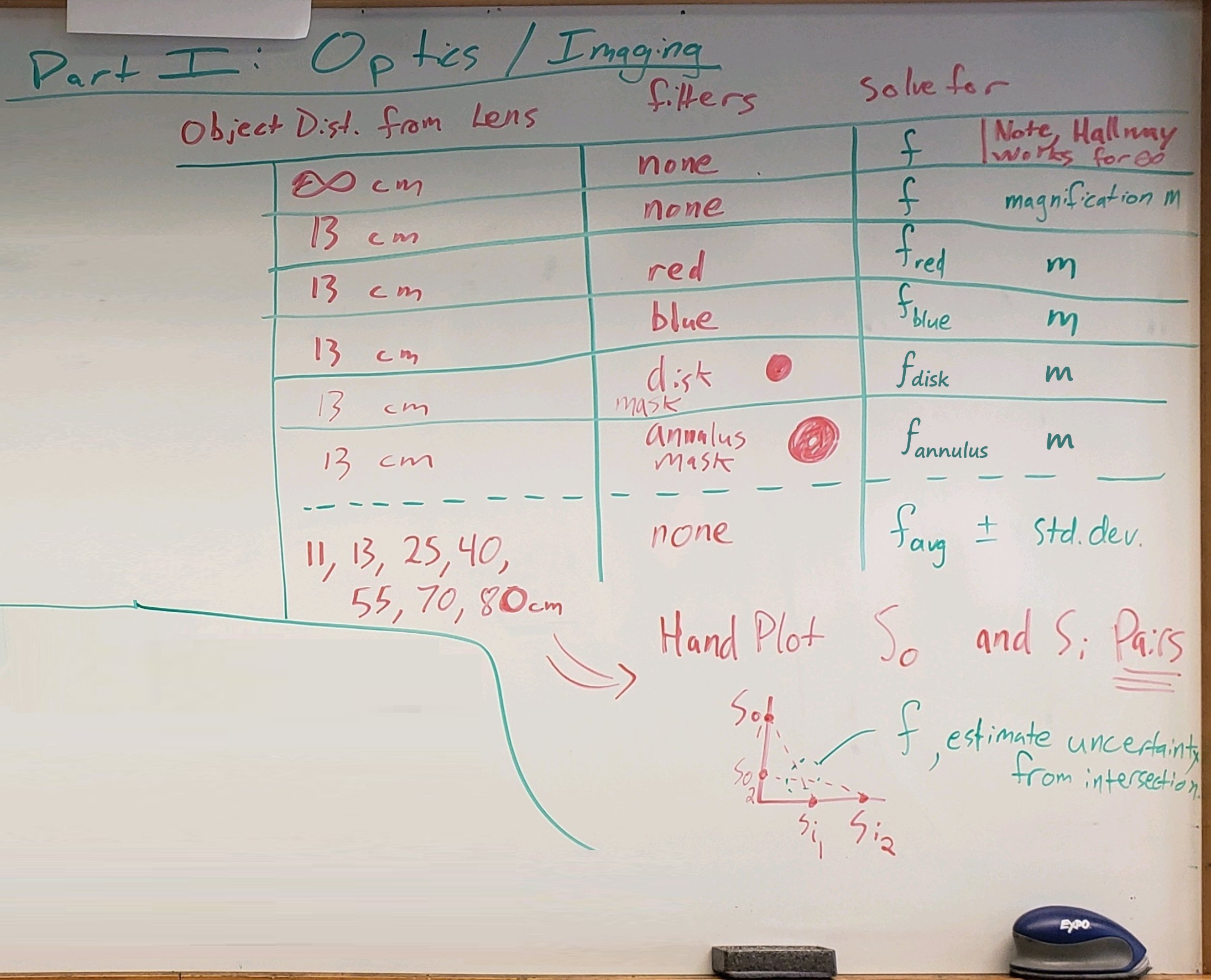
Fig. 143 Overview.#