Force Table with 3 Vectors at Equilibrium
Background
● Background Overview
There are two types of physical quantities: scalars and vectors. The number of attributes required to define a scalar and a vector distinguishes them. A scalar has just a magnitude telling us how large or small something is (or positive or negative); an example of a scalar quantity is temperature or speed (m/s)
A vector, meanwhile, is a quantity that is described by both a magnitude and direction. Examples of vectors are velocity (speed but with a direction; m/s at some angle) or force (a push or pull on an object with a specific magnitude at some direction).
A force vector example: a force may be 100 N in magnitude with direction 90° counterclockwise from the -axis. This force vector is written as 100 N @ 90°. We will use typefont of (with a note that bold isn’t always bold when viewing on some machines):
Vector --- bold, itallicised, with an arrow overhead ---
Scalar --- bold, itallicised with no arrow ---
Vector component --- bold, itallicised, with a subscript or --- or
When several vectors act on an object, it is generally desirable to determine the sum of these vectors, called the resultant vector. Suppose force vectors and act on a body. The resultant is defined by the vector sum of the two forces, thus
If many forces act on the body, then we sum all the forces together
The resultant force is a single force which can completely represent a number of individual forces acting. When the resultant force is zero, the object is said to be in equilibrium.
There are two methods of vector addition to consider:
The graphical method (reviewed here, but not conducted during lab today)
The method of components (conducted during lab today)
● Graphical Method
Vectors and (Figure 1) are added graphically as follows: Beginning at a convenient point on a piece of graph paper, usually at the origin of a rectangular coordinate system draw one of the vectors as an arrow to scale and pointing in the proper direction. Place the second vector with its tail at the tip of the first, again drawn to scale and pointing in the proper direction. The resultant is the vector drawn from the tail of the first vector to the tip of the second. The process is illustrated in Figure 2 demonstrating the addition operation does not depend on the order of addition. Thus, like scalar addition,
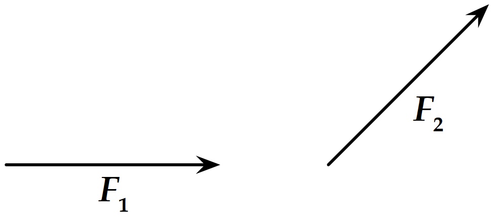
Figure 1:Two force vectors and
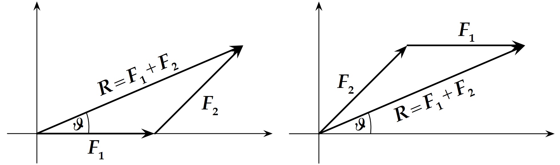
Figure 2:Adding 2 vectors and , using the graphical (“tail-to-tip”) method.
It is important that an appropriate scale be selected with which the vectors are drawn (e.g. 1 N = 10 cm). The magnitude of is determined using a ruler, and the angle is measured using a protractor. Since the negative of a vector is merely the vector pointing in the opposite direction, subtraction is addition with the negative vector pointing in the opposite direction. Errors can be significantly reduced by using a scale that makes the drawing as large as possible. Neatness counts!
● Method of Components
The method of components is a much more useful and quantitatively accurate method of vector addition. Each vector is resolved into components along the - and -axes. That is to say, the vector addition of the two components of the vector is the vector itself. Thus if two vectors are to be added, we add the components along each axis to form the components of the resultant.
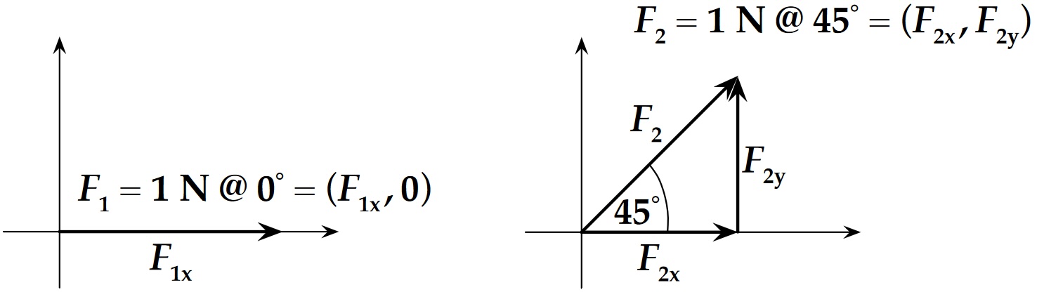
Figure 3:Adding 2 vectors and using the method of components.
In Figure 3, the magnitudes and directions are shown for the two force vectors and . The magnitudes of the and components are calculated for this example as follows:
Next, add the -components
Then, add the -components
The magnitude of the resultant is found using the relation
or
The angle specifies the direction of the resultant and it can be calculated by noting that
and
For this example illustrated in Figure 4
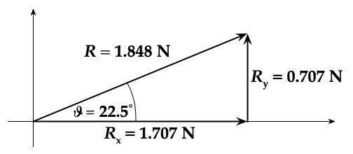
Figure 4:Example of , the sum of 2 vectors as - and -components, as well as its magnitude and angle with the -axis.
In this laboratory, an object will be presented with two known forces acting on it. Equilibrium will be established by adding a third equilibrant force , such that the sum of the three forces is zero (i.e. at equilibrium). Thus, we must first find the resultant of the two given forces and . Then we can determine the equilibrant, , equal in magnitude and opposite in direction to the resultant . This is illustrated in Figure 5.
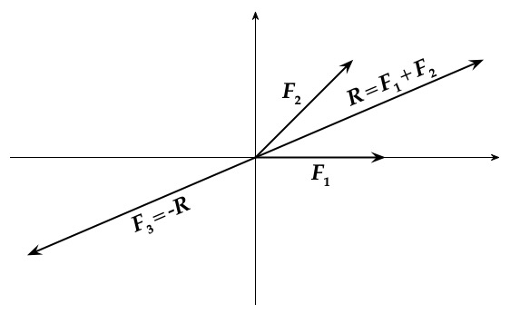
Figure 5:Illustration of the method to determine the force needed to balance two given forces and .
Here is the equilibrant force necessary to equilibrate and . Note that the resultant of all the vectors for today’s lab should add up to zero, i.e.
since the ring is in equilibrium.
Recall that , therefore the equilibrant force has the same magnitude as the resultant , but acts in a direction opposite to . So we now have
We conclude that the force necessary to equilibrate two or more forces is equal and opposite to the resultant of the two (or more) forces. This is additionally illustrated in an example of the force table apparatus we will use in Figure 6.
Apparatus
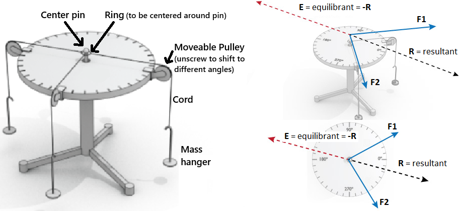
Figure 6:(Left) Illustration of the force table. (Right) An example of how to determine the force needed to balance two given forces and .
The apparatus for this experiment consist of a force table, weight holders, and weights (see Figure 6). The force table consists of a circular tabletop mounted on a vertical rod held in a tripod support with leveling screws. The rim of the circular top has a 360° scale engraved on it along which it is possible to clamp a number of pulleys. At the center of the table is a small ring held in place by means of a removable pin. The ends of three cords are tied to the ring with each cord leading over a pulley and ending with a weight holder tied to its other end. When the forces along the cords acting upon the small ring are balanced, or in static equilibrium, the ring remains stationary. For this lab, the force pulling on the ring is the tension of the string, which is merely translated from horizontal on the table to vertical.
Each hanging mass has an associated weight (force) due to being pulled down by gravity. This weight is balanced by the upward tension force of the vertical part of the cord which is merely translated from vertical to horizontal tension by the pulley. Thus, the force pulling the ring in the direction of the cord is
For accurate measurements of the angles involved, each cord must be aimed directly at the peg at the center of the ring requiring that the equilibrium condition must be established when the ring is exactly centered around the pin on the table. Use consistently the same counterclockwise protractor.
Experimental Procedure
● Preview & Examples
For today’s lab, two different cases will be assigned involving two given vectors and the determination of the equilibrant vector. A third case involves the determination of the mass of two unlabeled masses by balancing the system from a single known mass.
○ EXAMPLE --- Finding the Equilibrant (First two cases)
For each of the first two cases, you will have two given masses at given angles (direction). Each mass, consisting of a 50 g hanger plus the necessary additional mass, will be hung from a cord routed over a pulley at the assigned angular positions and finally tied to the ring. A third cord, hanger, and pulley assembly is put in place for the third, unknown force vector. Each force is the weight of the hanging mass at the pulley angle. Determine the unknown forces for each of the two cases.
If, for example, you were given the following case to work with
you would place a pulley at 0° and add 150 g to the 50 g weight hanger for a total 200 g. As mentioned in (15), the tension on the cord is the same on both sides of the pulley so that the downward pull of gravity on the hanger and masses is equal to the tension in the cord leading to the ring. Thus,
Similarly, add 200 g to a 50 g weight hanger and run its cord over a pulley mounted at 135°.
Having established the given magnitudes and directions for each of the given forces, and , you would adjust both the amount of mass hanging on cord 3 and its angular position so that the ring is stationary at the center of the table. In order for angular measurements to be accurate, each cord must be on a line that crosses through the center of the table. Sighting along each cord towards the center pin can help you to easily and accurately check this.
To determine the equilibrant vector experimentally , you will record both the angular position (direction) and total mass (to determine magnitude of the balancing force from the total hanging weight) required to balance and . You will then compare this vector to the expected vector based on your theoretical calculations.
○ EXAMPLE --- Determining 2 Unlabeled Masses (Third case)
In the third case, you will experimentally determine two unlabeled masses by balancing the and components of the force of a single known mass. Place the pulley with the known mass at . Experimentally determine the angles and for the unlabeled masses and that result in the ring being in equilibrium. For this case, assume angles and are actual values.
We can calculate the theoretical unlabeled masses using the method of components. You have to solve a pair of equations for the and components of force. The equation for equilibrium in the direction is
Similarly, the equation for equilibrium in the direction is
In these equations, we are assuming we know , , , , and that we want to determine and . Of the various ways your could do this, one way is to multiply (19) by and (20) by . The result is:
You can then subtract the component (22) from the component (21)
to find an equation where the only unknown is :
After algebraically solving for , you can use the known values to solve for the experimental and enter the value in your data table for later comparisons to the actual values.
After having algebraically solved for with (24), you could plug that equation back in to (22) to eliminate to find an equation where the only unknown is :
After algebraically solving for , you can use the known values to solve for the experimental and enter the value in your data table for later comparisons to the actual values.
You would then measure and on the scale and enter the values in the table and comare.
● CASE 1 & 2 -- Finding the Equilibrant Vector (Balancing Force)
Table 1:Case 1 & 2 Given Values
| Hanger (i.e. Vector) | Mass (g) | Angle (°) |
|---|---|---|
| Case 1 | ||
| 1 | 150 | 0° |
| 2 | 150 | 70° |
| 3 | ? | ? |
| Case 2 | ||
| 1 | 100 | 75° |
| 2 | 200 | 115° |
| 3 | ? | ? |
For these first two cases, with given initial values in Table Table 1, experimentally determine the 3rd (equilibrant) vector and compare your results to your expected values.
Create data tables for the first case. NOTE: The data layout for each of the first two cases is the same. Create for the first case and run the whole experiment, then you can copy/paste the same data table for the additional case(s).
Common data section with accepted value of (9.803 m/s²), mass of the hanger, list of slotted masses with their uncertainties (see table Table 2 later in the procedure), and any other common values. You will reference these values in the calculations.
An experimental data table (e.g. ● Case 1 & 2 Experimental Data) to record your experimental results with:
With three rows (1 for each of the 3 vectors).
Include columns for:
: hanging mass in kilograms (kg)
: your estimate of the experimental uncertainty [± value] of the masses in kg
: calculated magnitude of the force in Newtons (N)
: direction of the force vector in degrees
: your estimate of the experimental uncertainty of the angle in degrees
: calculated -component of each force vector in N
: calculated -component of each force vector in N
An analysis table (e.g. ● Case 1 & 2 Analysis - Resultant of Given Vectors & Experimental Total) to analyze the results of your measurements. This is effectively one row as there would be just a single value for each of the variables. The columns should include variables:
: the component of the resultant vector in N
: the component of the resultant vector in N
: magnitude of the resultant vector in N
: direction of the resultant vector in degrees
& : total of all vector components in N
: total overall magnitude of all vectors which we will also treat as in N
A secondary analysis table (e.g. ● Case 1 & 2 Analysis - Theoretical Values) to analyze your expected values. This is also effectively one row as there would be just a single value for each of the variables. The columns should include variables:
: your expected or theoretical magnitude of the equilibrant force in N
: theoretical equilibrant mass in kg
: theoretical equilibrant direction in degrees
Starting with the first case, add slotted masses to hangers 1 & 2 to set their masses equal to the given values in Table Table 1.
Loosen the screws of the black pulleys to rotate them around the tabletop to their given angles and retighten.
With hanger 3 (unknown vector), add or subtract slotted masses and scoot the pulley with hanger and masses around the force table until the system is at equilibrium.
Double check the given vectors are still lined up with their given angles. If not, readjust as needed.
Note your & values.
Also note both of your estimated uncertainties & .
For , estimate this based on the force table’s increments and your confidence that the ring is still centered on the center pin. Example: move the pulley left or right until you’re no longer convinced the ring is centered; however far you’ve shifted it, that will be your range.
For , add up the total uncertainty of each of your slotted masses. For today, assume each hanger is exactly 50 g, but the list of uncertainties for the slotted masses is below. Example: if you had measured 123 g from just slotted masses, you could have used one of each
100, 20, 2, 1 g, which would end up giving an uncertainty of g or g:Table 2:Slotted Masses
Mass (g) Uncertainty (g) 200 2.0 100 1.0 50 0.5 20 0.2 10 0.1 5 0.1 2 0.04 1 0.03
Calculate the hangers’ respective forces using (15).
Determine the hangers’ respective and components and . See (4).
In your analysis table, determine and , the and components of the resultant vector of this case’s two given force vectors and .
Determine the magnitude of the resultant vector (see Pythagorean Theorem in (7)).
Determine the direction of the resultant vector. See (10). Use the
ATAN2()Excel function to get the angle as measured counterclockwise from 0°.Determine & , the sum totals of the and experimental components from all of your vectors, i.e. and (see also (2), (5), (6), and (13)). Could also be stated as and .
Determine (also treated as ), the sum total experimental magnitude of all three of your vectors determined in similar fashion to (7), but with & .
In your secondary analysis table, based on the resultant of the two given vectors, determine your theoretical equilibrant vector that would balance the resultant, and its associated expected mass (see (14)):
magnitude
direction
mass
COMPARE your experimental results of hanger/vector 3 to the theoretical values. Does overlap (and therefore agree) with your theoretical value ? What about and ? If not, are there significant issues that may be contributing to the discrepancy? Discuss with instructor if so. To be further discussed in Section Post-Lab Submission --- Interpretation of Results.
Repeat for the second case (see Table Table 1) once you have completed the entire analysis procedure for Case 1 and are satisfied in your values and calculations.
● CASE 3 -- Determining 2 Unlabeled Masses
Table 3:Case 3 Initial Given Values
| Hanger (i.e. Vector) | Mass (g) | Angle (°) |
|---|---|---|
| Case 3 | ||
| 1 (empty, ) | 50 (just hanger, no extra masses) | 0° |
| 2 (Pikachu-black, ) | ? | ? |
| 3 (corgi-white, ) | ? | ? |
Experimentally determine the mass of just the Pikachu (black figurine) and the corgi (white figurine) and compare to actual values. The angles for hangers 2 & 3 will be treated as given values once experimentally determined. Reminder, the hangers are 50 g each.
Create data table for this case with columns for (e.g. ● Case 3 Data):
Experimental masses in kg
Given/actual angles in degrees
Actual values for each mass
The % Difference between the experimental and actual mass values in kg
Place the figurines on their respective hangers and set the empty hanger () to its initial angle found in Table Table 3.
Unscrew the black pulleys to rotate the figurines around the tabletop until you find equilibrium in similar fashion to the first two cases.
Once you’ve found equilibrium, record the given mass and angle as shown in the Table Table 3 for the empty hanger.
Record your experimentally determined angles & .
Determine & :
First algebraically solve (25) and (24) for and , respectively. Do this by hand before plugging the equations into your spreadsheet. There should be scratch paper and extra pens & pencils at the front of the room if needed.
Calculate your experimental masses for both figurines in your speadsheet using now your now solved equations. Reminders: hangers are 50 g, and there are trigonometric identities you could look up that could simplify the equations for your spreadsheet.
Measure and record the actual masses of each figurine, and , with a triple-beam balance.
COMPARE your experimental figurine masses to their actual values. Do they generally agree? Calculate the % difference of your experimental and to their actual measured values (see (26)). What may be contributing to a larger or smaller difference? To be further discussed in Section Post-Lab Submission --- Interpretation of Results.
Post-Lab Submission --- Interpretation of Results
● Finalized Spreadsheets
Make sure to submit your finalized data table (Excel sheet).
● Post-lab Writeup
In a paragraph, summarize your error analysis. Be both qualitative and quantitative.
What are the uncertainties of Cases 1 & 2 (Finding Equilibrant)?
What is the precision of your equipment (force table, masses, etc.)?
What are possible systematic (affecting accuracy) errors of the experiment? What are possible random (affecting precision) errors?
Return to results section question: ‘‘In other words, for each of the first two cases, COMPARE your experimental results of hanger 3 to the theoretical values for hanger 3.’’ How does changing by and by change ? Do the math in your spread sheet.
What uncertainties might make the difference between your final results and expected values larger or smaller? Is there any source of uncertainty that contributes the most variability of ?
For Case 3 (Unlabeled Masses), what errors may contribute to larger or smaller % differences to the actual measured-by-triple-beam-balance values?
In a paragraph, summarize the results you have determined in each case, i.e. ... and answer the following questions (longer does not mean better):
What is a vector?
What is the physics behind balancing your vectors today?
Case 1 & 2 (Finding Equilibrant):
Looking at your experiment, why do the two given masses not add up to the third mass?
What are your results, and how do they compare to the theoretical predictions?
In other words, for each of the first two cases, COMPARE your experimental results of hanger 3 to the theoretical values for hanger 3.
Does the vector magnitude overlap (i.e. agree) with your theoretical value ?
Does overlap with your theoretical value ?
Does overlap with your theoretical value ?
Case 3 (Unlabeled Masses):
How do your values for and compare to your actual values from the triple-beam-balance?
What is the percent difference between your experimentally determined masses and their actual measured values? Calculate the % difference in each of the masses using the following relation (Note: If you change the Excel number format of this cell to
Percentage, do not multiply by 100 as Excel will do that for you):
The Whiteboard
Example data tables are shown below to assist you in building your spreadsheet for this lab. Additionally the original whiteboard summary is at the end of this section.
● Case 1 & 2 Experimental Data
| Hanger/Vector | (SI units) | (SI Units) | (SI Units) | (°) | (°) | (SI Units) | (SI Units) |
|---|---|---|---|---|---|---|---|
| 1 | |||||||
| 2 | |||||||
| 3 |
● Case 1 & 2 Analysis - Resultant of Given Vectors & Experimental Total
| (SI units) | (SI Units) | (SI Units) | (°) | (SI Units) | (SI Units) | treated as (SI Units) |
|---|---|---|---|---|---|---|
● Case 1 & 2 Analysis - Theoretical Values
| (SI Units) | (°) | (SI Units) |
|---|---|---|
● Case 3 Data
| Vector | (SI units) | (°) | (SI units) | % diff. masses |
|---|---|---|---|---|
| 1 (known) | ||||
| 2 (Pikachu-black) | ||||
| 3 (Corgi-white) |
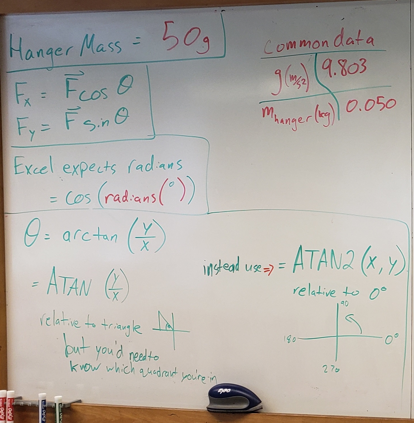
● Original Whiteboard Info