1145L-ONLY | Ideal Gas Law with Isothermal & Adiabatic Compression; Estimating Absolute Zero
Background
● Background Overview
A general and complete description of an ensemble of many atoms or molecules is a very difficult, if not impossible task, given the large number of objects involved. Luckily enough most gases follow a relatively simple approximation for a rather large range of conditions.
The ideal gas law describes the behavior of a gas of point-like particles. While there is no such thing as an ideal gas (all real molecules have a small but non-zero size), it is nevertheless a good approximation to the behaviour of gasses at ordinary temperatures and pressures.
● Ideal Gas Law
The Ideal Gas Law assumes that
The gas is made up of molecules moving in straight lines, but random directions,
All collisions between the molecules themselves and between the molecules and the walls of the container are perfectly elastic,
The temperature of the gas is directly proportional to the kinetic energy of the molecules,
The pressure of the gas is due to the collisions of the molecules with the walls of the container,
All inter-molecular forces can be neglected, and
The volume occupied by the molecules is negligible as compared to the volume of the container.
Under these conditions the pressure, temperature, and volume of the gas will follow a simple relationship,
where is the gas pressure in Pascals (1 Pa = 1 N/m²), is the gas temperature in Kelvin, is the volume (in m³), and is the number of moles in the gas (1 mole = 6.022×10²³ molecules). is called the universal gas constant and for these units has the value J/(mol·K).
Most gases will behave approximately as an ideal gas within a certain range of conditions across a number of different types of processes, but the law fails at low temperatures or higher pressures when forces between the gas molecules become important.
For today’s lab, the two processes we will focus on are
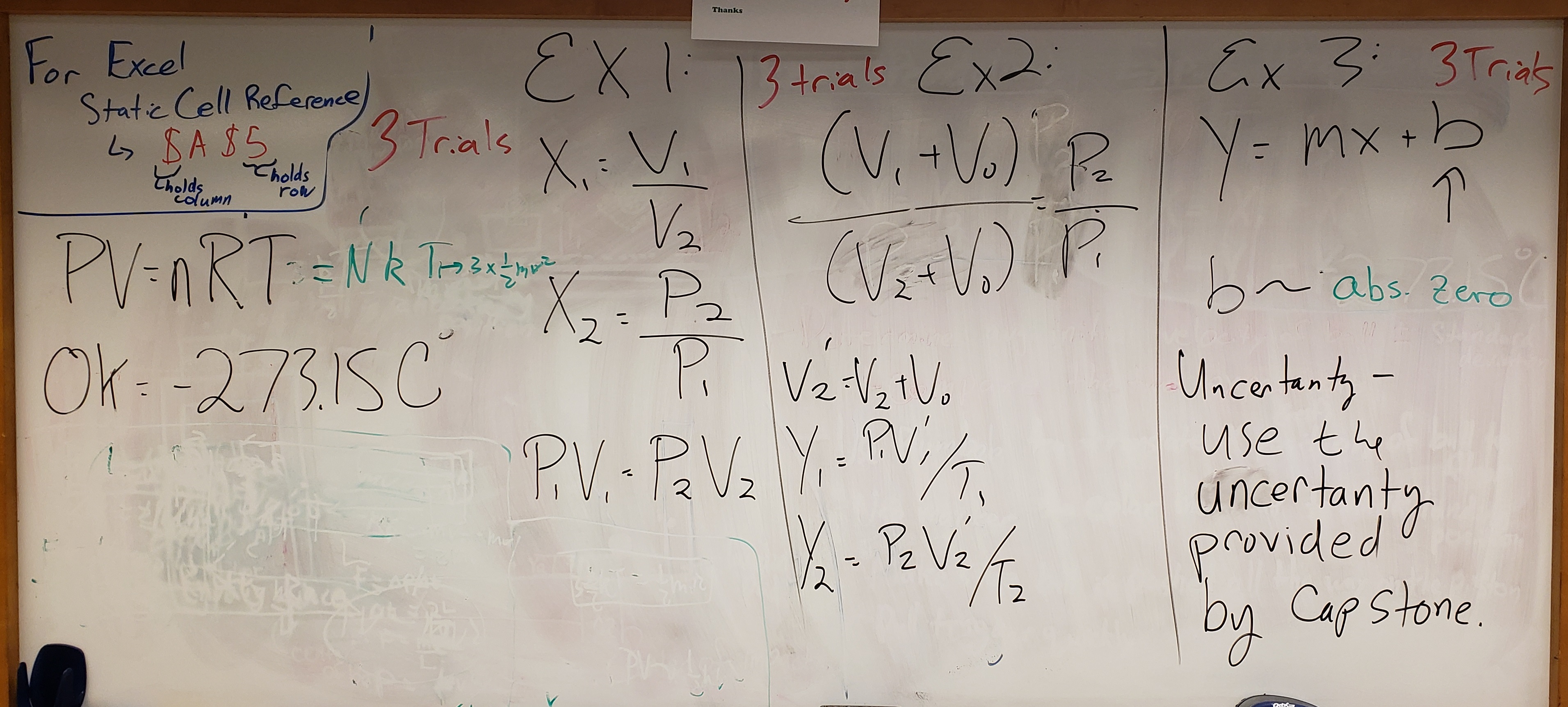
Isothermal: temperature is kept constant through the process (e.g. a process analyzed when initial temperatures are the same as the final temperatures). This is possible when the ratio is kept constant.
Adiabatic: energy of the system is kept constant (i.e. the parcel of gas does not exchange or lose energy to its surroundings). This is possible when the ratio is kept constant.
● Absolute Zero
One of the things the ideal gas law assumes is that the kinetic energy of the gas molecules is directly proportional to the temperature of the gas. Therefore, if the molecules have no kinetic energy (the molecules are at rest) then the temperature of the gas is at its lowest possible value. This temperature is called absolute zero and is used as the zero-point of the Kelvin temperature scale
Note that, according to the definition of pressure, gas molecules at absolute zero will also exert no pressure on the walls of the container the gas is in.
● Experimental Equipment Review
This experiment uses temperature and pressure sensors plugged into an interface so that data for both variables can be recorded simultaneously. For the Ideal Gas Law experiment the air inside a syringe is compressed by pushing on the plunger. Pressure and temperature values are collected and recorded with the Capstone program, which is then also used to analyze the data. For the Absolute Zero experiment a hollow sphere (with a fixed volume) is submerged in liquids of different temperature. Capstone will again collect and record pressure and temperature data of the gas enclosed in the sphere. Pictures of the experimental setups are shown in Figure 1, Figure 2,and Figure 3.
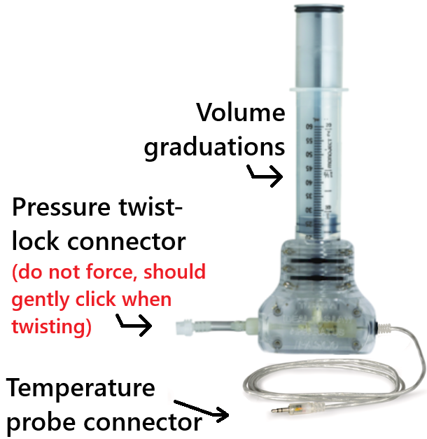
Figure 1:The picture shows the Ideal Gas Law experimental apparatus. The two cables coming from the syringe are the temperature and pressure connectors. The plunger of the syringe has a mechanical stop to prevent full compression of the syringe. Note: be gentle with the pressure connector; you need to insert and gently twist to lock it in place. DO NOT FORCE IT.
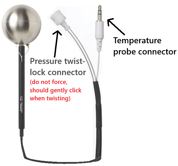
Figure 2:The picture shows the Absolute Zero experiment. The pressure and temperature connectors are shown exiting at the end of the black cable of the device. Note: be gentle with the pressure connector; you need to insert and gently twist to lock it in place. DO NOT FORCE IT.
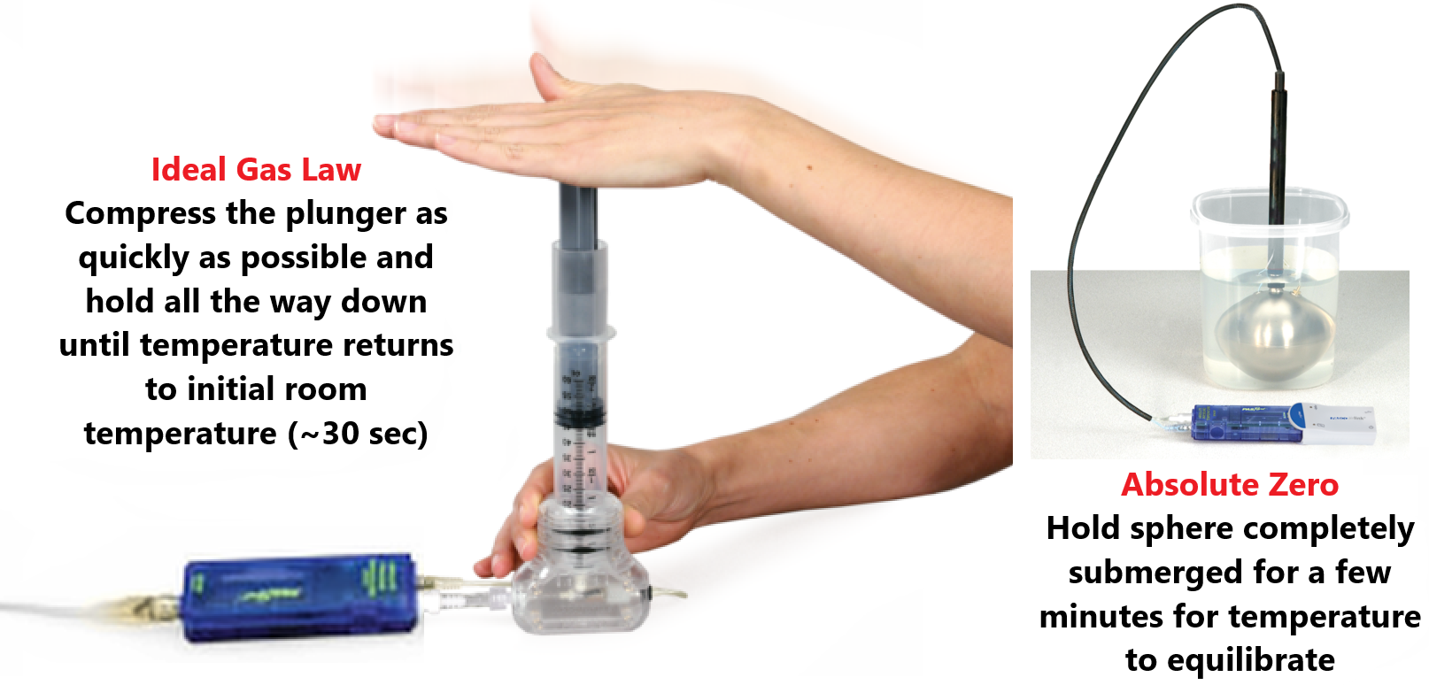
Figure 3:This picture shows the experimental methods for the Ideal Gas Law (left) and Absolute Zero (right) experiments. In both cases the temperature and pressure connectors are plugged into the PasPort Absolute Pressure Temperature Sensor (the small blue box).
Experimental Procedure --- Thermodynamic Processes
● Preliminary Data Acquisition
Create a data table for your ideal gas law measurements and calculations for your isothermal analysis including, but not limited to:
Measured values
Calculated ratios
Open graphs of absolute pressure (-axis) vs. time (-axis) and temperature in Kelvin (-axis) vs. time (-axis) in the Capstone program. Also have a table displaying absolute pressure and temperature open. All these can be opened by double-clicking on the corresponding items on the right-had side of the Capstone program.
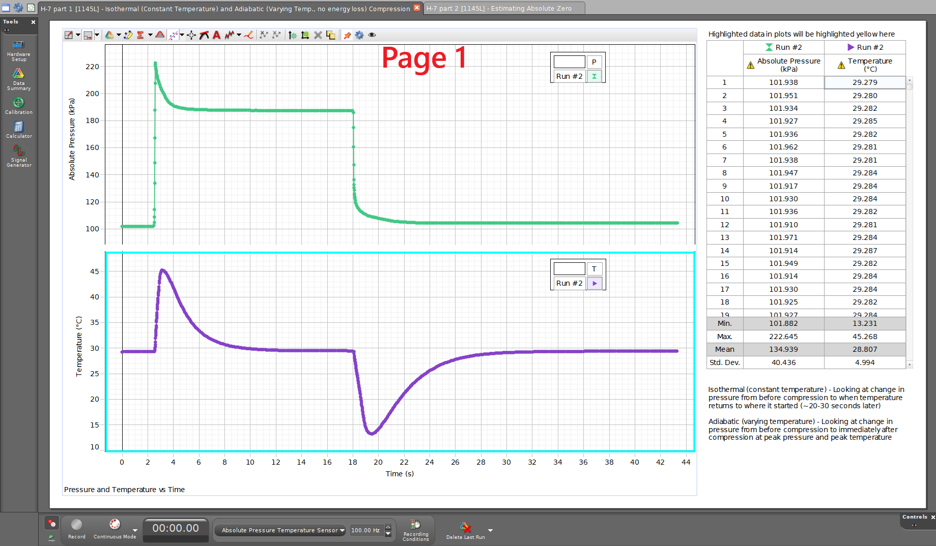
Figure 4:Example of Page 1 in today’s Capstone file for the different theromdynamic processes.
Disconnect the quick-release pressure connector and push the plunger all the way down. Note that the mechanical stop will prevent the plunger from being pushed all the way to the bottom of the syringe. Record the volume reading on the syringe as the volume in your Part 1 Data Table. The value for should be about 20 cc.
Set the plunger for an initial volume of cm³.
After you have adjusted the volume, re-connect the pressure port.
Hold the base of the syringe firmly against a sturdy, flat surface (the lab table).
Press the Record button on Capstone.
Press straight down as hard as you can on the plunger with the palm of your hand to fully compress the gas inside the syringe. Keep pressing to hold the pressure steady. Important: Do not let the pressure drop for at least 30 s. The mechanical stop will prevent you from decreasing the volume of the gas to less than than about 20 cc. Hold this position until the temperature and pressure have stabilized and are no longer changing (use the data table as an indicator). It should take less than 30 seconds for the temperature to return to room temperature.
Release the plunger and allow it to expand back out on its own (it may not go back to 40 cm³). Wait again until the temperature and pressure have equalized and are no longer changing.
Press the Record button again on Capstone to stop recording data.
● Analysis Part I --- Constant Temperature (Isothermal)
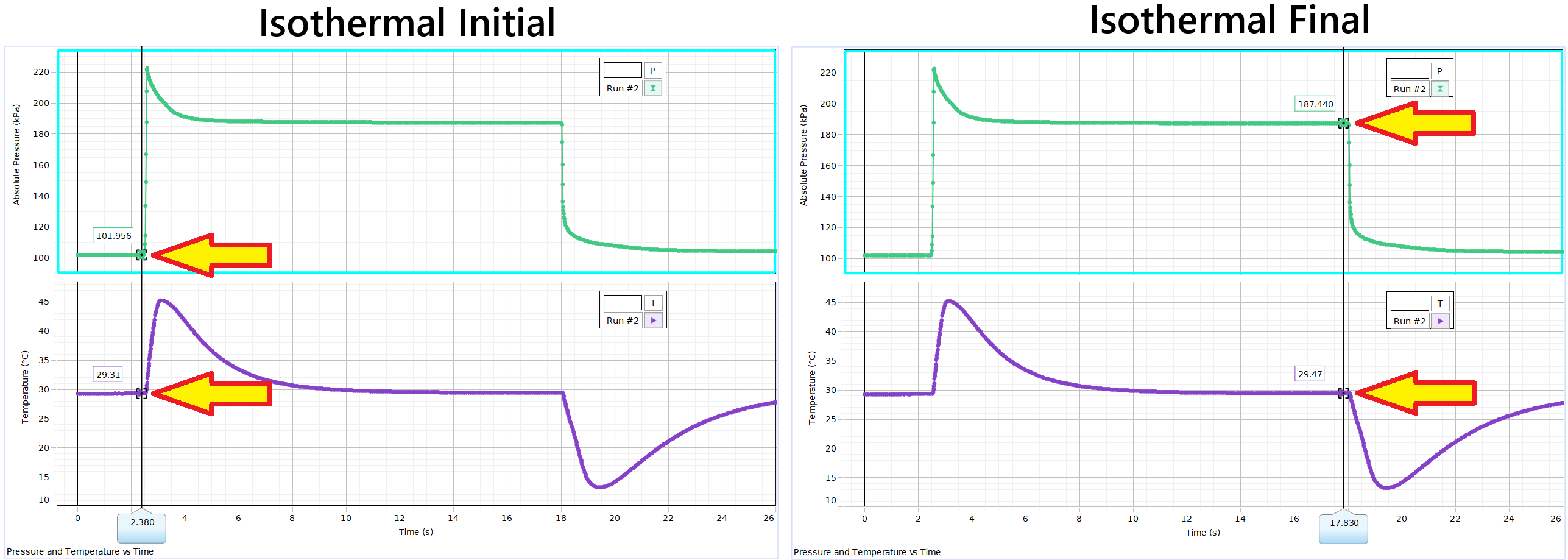
Figure 5:Example of initial and final pressure and temperature locations for the isothermal process.
Highlight an area (click and drag with the mouse) on the pressure graph at the beginning of the data-collecting run, before you compressed the air in the syringe. The highlighted values of the selected data points will appear in the data table of Capstone. Record the initial pressure as in your Part 1 Data Table.
Highlight an area on the pressure graph at the point just before you released the plunger. Record the final pressure as in your Part 1 Data Table.
Calculate the ratio of initial volume over the final volume, and record the result in your Part 1 Data Table.
Calculate the ratio of final pressure over the initial pressure, and record the result in your Part 1 Data Table.
Compare the two ratios. According to the ideal gas law (1) the two values should be equal, since for constant temperature (note that the temperature is room temperature in both cases). Discuss, first amongst yourselves and then with your instructor, why the values are different.
By now you have (hopefully) figured out that you have not accounted for the small amount of volume of air inside the tubing of the apparatus. Using the ideal gas law (1) and the data you collected in part 1, you can actually calculate this volume by solving the following equation for
Using the data from your first data table, calculate the value for and note the result for use in your upcoming data table.
Take a screenshot/photo of your graph --- 1 set of Pressure vs. Time & Temperature vs. Time plots representative of the Isothermal Compression. Note which locations on the plot you are using for your measurements. Adjust axes as necessary.
● Analysis Part II --- Varying Temperature and No Energy Loss (Adiabatic)
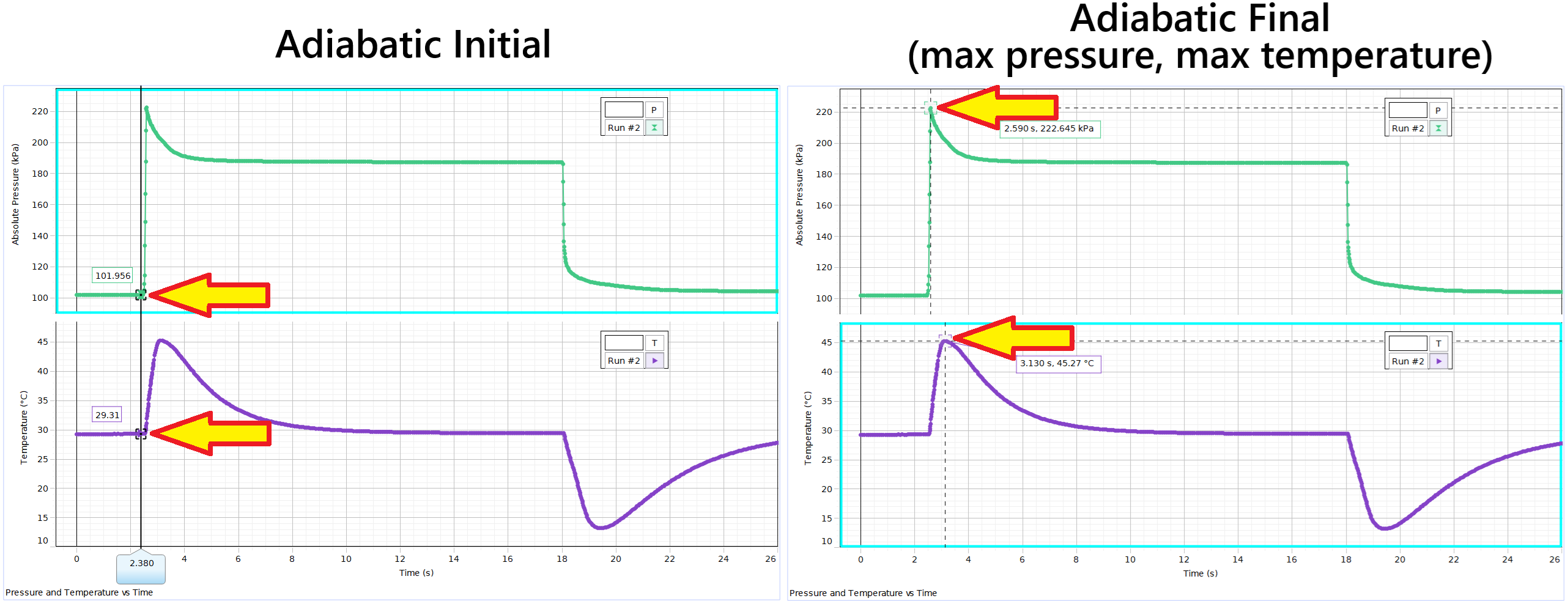
Figure 6:Example of initial and final pressure and temperature locations for the adiabatic process. Note: the temperature sensor lags slightly behind the pressure sensor, focus on the peak or max values when necessary. The quicker you compress the syringe, the closer in time the pressure and temperature peaks will be.
Create a second data table for your ideal gas law measurements and calculations for your adiabatic analysis including, but not limited to:
Measured values
Calculated values
Highlight an area (click and drag with the mouse) on the temperature graph at the beginning of the data-collecting run, before you compressed the air in the syringe. The highlighted values of the selected data points will appear in the data table of Capstone. Record the initial pressure and the initial temperature as and in your Part 2 Data Table.
Note the initial volume in your Part 2 Data Table.
Highlight the area (click and drag with the mouse) on the temperature graph where the temperature peaks. The highlighted values of the selected data points will appear in the data table of Capstone. Note the peak temperature and the corresponding pressure at this instant as and in your Part 2 Data Table.
Note the volume in your Part 2 Data Table.
Calculate the ratio and record the result in your Part 2 Data Table.
Calculate the ratio and record the result in your Part 2 Data Table.
Assuming the most significant error is in the volume, compare the difference between the two ratios with your estimate of the uncertainty in the volume.
Return to ● Preliminary Data Acquisition to repeat the previous steps for additional trials.
Create additional rows in your data tables for average and standard deviation calculations of your data for comparisons for each of the thermodynamic processes.
Take a screenshot/photo of your graph --- 1 set of Pressure vs. Time & Temperature vs. Time plots representative of the Adiabatic Compression. Note which locations on the plot you are using for your measurements. Adjust axes as necessary.
Experimental Procedure --- Absolute Zero
Create a third data table for the measurement of absolute zero including, but not limited to:
the pressure and temperature you measured at the hot, warm, and cold temperatures
-intercept and the accepted value of -273.15°C
Connect the Absolute Zero apparatus to the PasPort Absolute Pressure Temperature sensor (both the temperature sensor and the quick-release pressure port need to be connected, see Figure 2 and Figure 3-right).
Switch to the second page in your Capstone file (see Figure 7)
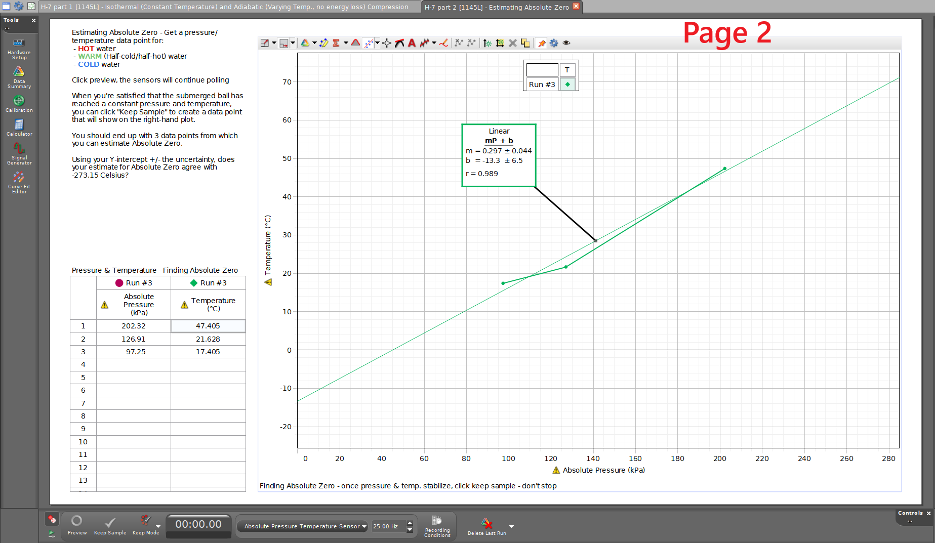
Figure 7:Example of Page 2 in today’s Capstone file for the absolute zero estimation.
Click on the Preview button to start collecting data. The data from the sensors will continuously update, but not save any data point until you press the Keep Sample button in the following steps.
Run the hot water until steam rises from the sink. Fill a pitcher to the 2 quart mark.
Hot --- First fully submerge the sphere in hot water (see Figure 3-right): Observe the data points appearing on the graph. Make sure the sphere stays completely submerged the entire time you take data. Once the temperature has reached equilibrium (i.e. the value in the digital display no longer changes), press the Keep Sample button (Do NOT stop the data collection by clicking on the red square button again). Read and note the values for pressure and temperature in your data table.
Warm --- Next remove half of the water in your container and replace it with cold water from the sink to get warm water. Again fully submerge the sphere in the water and make sure the sphere stays completely submerged the entire time you take data. Note how the point moves in the Temperature vs. Pressure graph as the values change. Discuss the outcome among yourselves and with your instructor. Once the temperature is stable again (this will take a few minutes) press the Keep Sample button again. Read off and note the values for pressure and temperature in your data table.
Cold --- Finally submerge the sphere in the cold water. Once again you need to make sure the sphere is completely submerged during the time you take data. Note how the point moves in the Temperature vs. Pressure graph as the values change. Discuss the outcome among yourselves and with your instructor. Once the temperature is stable again (this will take a few minutes) press the Keep Sample button again. Read off and note the values for pressure and temperature in your data table.
Press the Stop button to stop recording data.
Using the fitting tool in Capstone, fit a straight line to the 3 data points you have taken.
The -intercept of the best-fit line is the value for absolute zero temperature. Discuss among yourselves and with your instructor why this is the case. Note the result as in your data table.
Compare your result to the accepted value of -273.15°C.
Take a screenshot/photo of your graph --- 1 of Temperature vs. Pressure plot with axes scaled to see y-intercept(full absolute zero extrapolation). Note which locations on the plot you are using for your measurements. Adjust axes to show , i.e. the y-intercept.
BEFORE CLOSING CAPSTONE:
BEFORE LEAVING LAB:
Post-Lab Submission --- Interpretation of Results
This week’s lab is built of essentially two different, but still related to thermodynamics, experiments. To assist in your analysis and writeups, the suggested talking points below are broken up into the Thermodynamic Processes and Absolute Zero parts of the lab. You will still have single document for error analysis and single document for results as assignments in Blackboard.
● Finalized Spreadsheets
Make sure to submit your finalized data table (Excel sheet).
Please include relevant screenshots of your Capstone plots including:
1 set of Pressure vs. Time & Temperature vs. Time plots representative of the Isothermal Compression
1 set of Pressure vs. Time & Temperature vs. Time plots representative of the Adiabatic Compression
1 of Temperature vs. Pressure plot with axes scaled to see y-intercept(full absolute zero extrapolation)
● Thermodynamic Processes Post-Lab
In a paragraph, summarize your error analysis. Be both qualitative and quantitative.
What are possible random errors for today’s experiments?
What are possible systematic errors for today’s experiments?
Constant Temperature (Isothermal):
What may cause a discrepancy between the ratios of volumes and pressures?
Varying Temperature (Adiabatic):
What may cause a discrepancy between the ratios of volumes, pressures, temperatures?
Consider the uncertainty due to volume; do the ratios agree within that uncertainty range?
In a paragraph, summarize the results you have determined in each case. Consider:
Constant Temperature (Isothermal):
How do the two ratios, and , compare?
What is the percent difference between the two ratios?
Do your average ratios ± standard deviations agree?
What properties of a system must be proportional if compression is isothermal?
Assuming your ratios are comparable for the isothermal process:
What properties of the system changed, and how did they change?
What assumption do we make for an isothermal process (i.e. were there properties of the system that didn’t change)?
If your ratios did not agree, why?
Varying Temperature (Adiabatic):
How do the two ratios, and , compare?
What is the percent difference between the two ratios?
Do your average ratios ± standard deviations agree?
What properties of a system must be proportional if compression is adiabatic?
Assuming your ratios are comparable for the adiabatic process:
What properties of the system changed, and how did they change?
What assumption do we make for an adiabatic process (i.e. were there properties of the system that didn’t change)?
If your ratios did not agree, why?
● Absolute Zero Post-Lab
In a paragraph, summarize your error analysis. Be both qualitative and quantitative.
What are possible systematic errors for today’s experiments?
How did you determine your uncertainty in your absolute zero value?
How may systematic errors affect your determined value for absolute zero (i.e. increase or decrease)?
In a paragraph, summarize the results you have determined in each case. Consider:
What is your extrapolated result for absolute zero including uncertainty range? How does it compare to the accepted value?
What does absolute zero represent about a system?
The Whiteboard