Determination of Acceleration due to Gravity, g, with Simple Pendulum
Background
● Background Overview
In this lab, the acceleration due to gravity is determined by measuring the parameters of the nearly simple harmonic motion of a simple pendulum. The construction of the pendulum and restrictions on the motion of the pendulum permit some simplifying assumptions to be used to derive a relationship for in terms of easily measured parameters.
The gravitational attraction of the Earth on any massive body provides a force, which can accelerate a mass free to move under the influence of this force. This acceleration is dependent on the mass of the earth and inversely on the distance of the mass from the center of the earth. The value of is usually assumed to be constant over small vertical distances, i.e. distances that are small with respect to the distance to the center of the earth. Thus we will compare our results to the accepted value of at in Fairfield, CT ().
A pendulum is a massive body suspended such that it can swing freely. In the general case, the mass of the pendulum is an extended mass and is called a physical pendulum. An example of a physical pendulum might be a long piece of lumber, which is suspended from a nail through a hole near one end of the wood. This pendulum, when displaced sideways from its rest position, will swing back and forth under the influence of gravitational force which acts to restore the pendulum to its stationary hanging position. The harmonic motion of the swinging pendulum must be analyzed carefully by considering torque on the pendulum and the pendulum’s inertia. The torque is the turning force produced by gravity and its inertia is the total effect of all the mass parts of the pendulum resisting rotation around the pivot. The torque and inertia are exactly analogous to force and mass in the linear motion case described by Newton’s Second Law, .
When all of the mass of the pendulum can be considered at a common distance from the pivot, then the physical pendulum is a simple pendulum. An example of a simple pendulum is a relatively small, massive object suspended from a long, nearly massless connection to a pivot like a short, heavy bolt, tied to a pivot with a thin thread.
Under the assumption of a simple pendulum, the analysis of the motion can be carried out using Newton’s Laws of Linear Motion that we have seen in class. Figure 1 illustrates a simple pendulum at some arbitrary point in its swinging motion back and forth. We define this point by the angle of the thread with the vertical, indicated by the dashed line. The forces acting on the mass are its weight straight down and the tension in the thread. The weight can be resolved into a component along the direction of the thread and a component perpendicular to the thread, i.e. along the tangent of the arc of the swing.
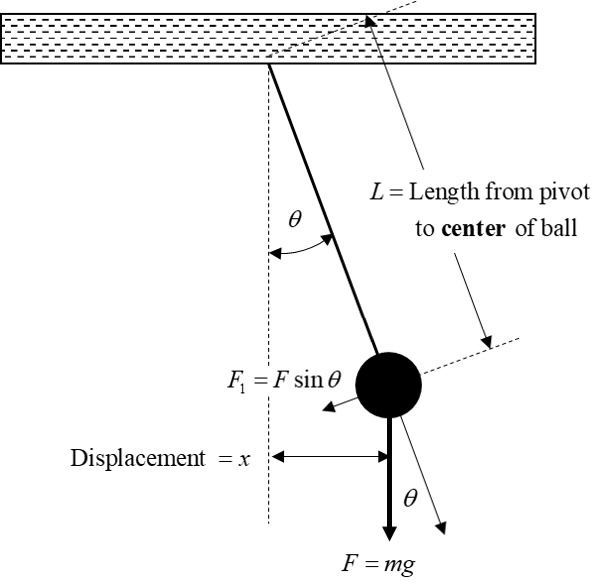
Figure 1:Force Diagram and variables used in the pendulum experiment.
, the force along the direction of motion, is equal to . We will now make a further simplifying assumption which is to assume that the maximum angular displacement, i.e. the maximum value of , is small. If the value of , and therefore , is small, then the magnitude of both the and are essentially equal to , measured in radians.
The implication of this small-angle assumption is that the pendulum never swings very far from the vertical. Therefore the restoring force, i.e. the force that is acting to return the pendulum to its equilibrium vertical position, is assumed to be acting horizontally. This is clearly never true except at the equilibrium position where the restoring force is zero. The implication of this assumption is that the actual restoring force is always less than the value we assume it to be.
The period of the pendulum is the time it takes to swing through a complete cycle, or one complete swing out and back to the starting point. Using the small angle assumption described above, we can write the restoring force as
The minus sign means that the restoring force is in the opposite direction from the displacement . When the restoring force of a system is of the form , the system will oscillate in simple harmonic motion.
To see what this motion looks like we will use Newton’s Second Law,
where is the acceleration of the mass in the -direction.
Substituting the definition of acceleration
into (2) yields an equation for displacement, , as a function of time, , namely
Upon simplifying, the mass, , disappears, yielding
This second order, linear, differential equation has a solution
where the amplitude is the maximum value of ; is the period; and the motion is such that at , the pendulum is at its maximum displacement, i.e. . Note that the motion is independent of the mass. Substitution of this solution into the differential equation yields an expression for the period of a small-amplitude pendulum as
Rearranging this expression we can similarly obtain a small-amplitude-approximated value
and, for our uses of plotting our experimental data later on,
Had we not constrained the motion of the pendulum to small amplitudes, the expression for the period would be given by the small-amplitude approximation multiplied by an infinite Taylor Series of additional, smaller correction terms
Thus as the angle gets larger, the period increases as those additional terms become significant. You can see example of this by the slightly longer period of the large angle example in ● Demo Video: Counting & Small vs. Large Angles.
For our uses today, we will only focus on the first three terms of the Taylor Series, and call everything in the brackets our Taylor Series correction factor, denoted as , such that
simplifies our equation for the period to
When the pendulum swings with very small angles, the period is essentially independent of the amplitude. However, from the more precise expression above for the period, this is not strictly true. An amplitude decrease could result from the effects of friction in the pivot or air drag of the thread and mass. Pendulum clock makers go to great pains to not only keep the length constant, but the amplitude of the swing as well. Since we will average over many cycles, we must also assume that the amplitude does not change as we measure the period. In our experiment, we might be tempted to average a very large number of cycles to reduce measurement errors. However the necessarily larger initial amplitude together with the decreasing amplitude caused by friction effects would change the average period. For the last case, we will do just that by deliberately starting with a large amplitude and observe whether there is an increase in the measured period.
Experimental Procedure
● Procedure Preview
● Preliminary Setup
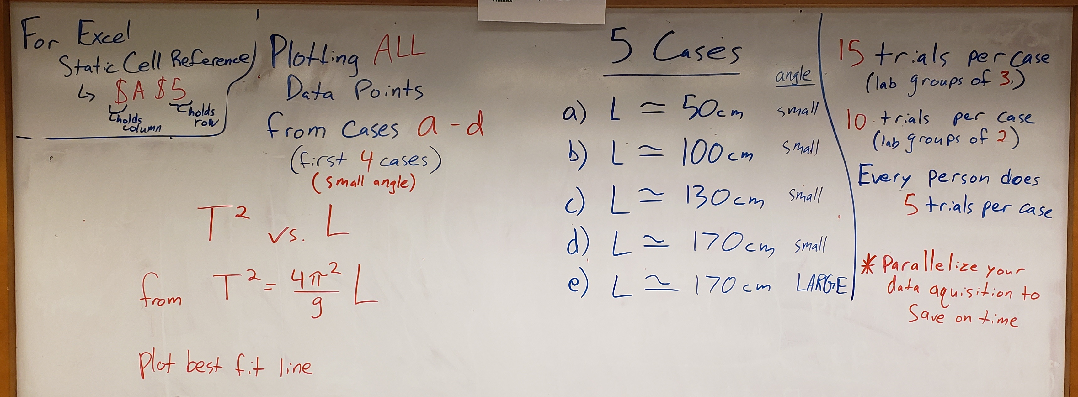
Five Cases: For this experiment, you will use approximate pendulum lengths as listed in Table 1. You don’t have to set the lengths to be exactly those lengths. The point here is to cover a wide range to investigate how the motion is dependent on pendulum length. Get close and make sure to measure the thread length carefully; record the measured value, and determine the total pendulum length for the given case. For each case, perform the following steps listed in ● Experimental Data Collection and record the data appropriately in your spreadsheet.
Table 1:Five experimental pendulum-length cases
Case Rough Pendulum Length Angle Size 1 50 cm small 2 100 cm small 3 130 cm small 4 170 cm small 5 170 cm LARGE NOTE ON NUMBER OF TRIALS: For each of the five cases, each person will perform 5 time trials. Everyone can record at roughly the same time, but don’t worry if you aren’t all timing the exact same swings (i.e. someone starts a half or whole cycle late); just make sure to time a total of 10 cycles for each trial. By everyone taking data for 5 time trials each, and doing so simultaneously, a two-person group will end up with 10 total data points, and a three-person group will have 15 total data points for each case, etc. while saving time running the lab.
Create a data table for the given case (this table can be copied/pasted for the additional cases):
Common data for the entire experiment including the ball radius and the accepted for Fairfield.
Common data for each individual case including:
The case number
The case description
: Measured thread length
: Calculated pendulum length
: Estimated uncertainty in length
: Approximate angle of displacement
Data table including, but not limited to:
Enough rows to include all time trials for your group
For each case, include columns for
Trial number
Lab member’s initials
: Measured total time of the 10 cycles (swing out and back to initial position)
: Estimated uncertainty in total time
: Period of a single swing as determined from your measured time
: Uncertainty of the period similarly determined from
: Experimental value of small-amplitude-approximated acceleration due to gravity
: Uncertainty of small-amplitude-approximated experimental value from error propagation
: Magntitude of difference between and the accepted , i.e. how far away your small-amplitude-approximated value is from the accepted value of
: Taylor Series correction factor
: Corrected value of by incorporating the additional terms of the Taylor Series correction factor that increases the period
: Magntitude of difference between and the accepted , i.e. how far away your corrected value is from the accepted value of
Include an additional row for summarizing your results including, but not limited to:
: Average from all trials of the current case
: Average small-amplitude-approximated from all trials of the current case
: Average uncertainty of from all trials of the current cases
: Average magntitude of difference between and the accepted
: Average corrected values of
: Average magntitude of difference between and the accepted
: Slope-derived value of from fitting a trend line to all small-amplitude data points
: Uncertainty of slope-derived value of , found by propagating the uncertainty of the slope of the fit
: Magntitude of difference between and the accepted
Include an additional section for plotting and analysis
Columns for all and values from all small-amplitude trials across all relevant cases combined together for easy plotting
Section for
LINESTfunction. Must be an empty 2 column 5 row section in your spreadsheet as those cells will be autopopulated by theLINESTfunction later on. Used for determining the slope and the slope’s uncertainty
The total pendulum length can be determined from adding together the thread length and the ball radius:
Measure the thread length . Attach one end of the thread to the provided pendulum clamp in such a way that you can accurately measure the distance from the pivot point to the top surface of the ball. Set the length of the thread approximately to the value for the case (doesn’t have to be exact, we’re just looking to test across a range of lengths across the cases).
Measure the diameter of the ball with Vernier calipers, determine its radius, add the radius of the ball to the thread length to establish the pendulum length .
Estimate and note the uncertainty in the pendulum length ; consider both each measurement tools’ precision as well as your estimated confidence in your measurements (i.e. are you as confident as the tools’ precision, or might it be a bit of a larger range?).
Note the approximate angle of displacement from rest position:
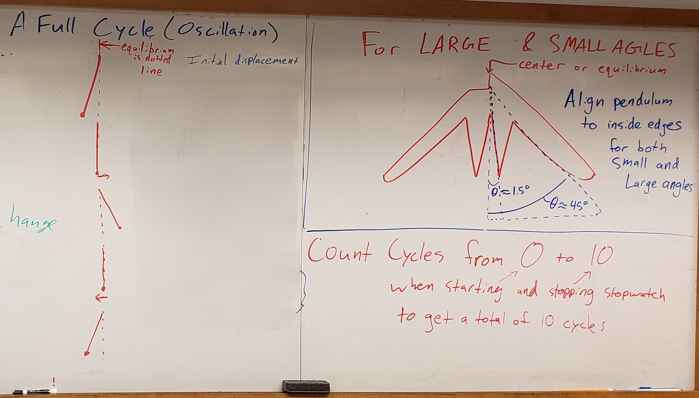
For cases 1--4, the starting displacement should be small (e.g. from the inner edge of the narrow arm of the red protractor).
For case 5, use a large angle (e.g. from the inner edge of the wide arm of the red protractor).
● Demo Video: Counting & Small vs. Large Angles
Demonstration video: shows suggested counting procedure by starting your counting on 0 so when you reach 10, you've counted 10 full cycles. Example of this is presented for both small and large angles. Also shown is the effect of a large angle on a pendulum, increasing the period and causing a pendulum of the same length to become out of sync with the small-angled pendulum.
● Experimental Data Collection
For each case, perform 5 trials per person (i.e. 10 or 15 total data points per two- or three-person group as mentioned above) as follows:
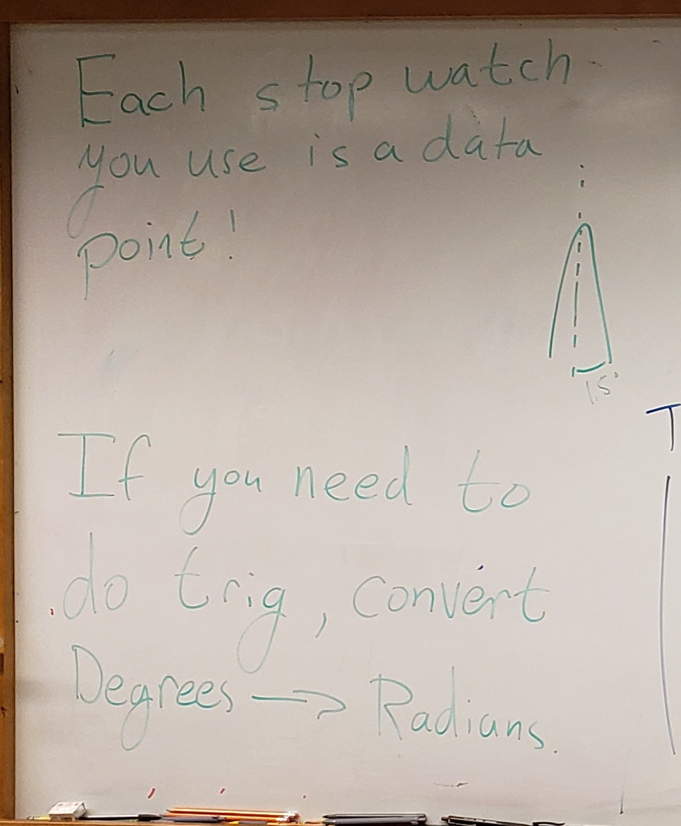
Measure the time for 10 cycles of the pendulum. One cycle is going from the pendulum’s initial position, swings out, swings back to its initial position. See example in ● Demo Video: Counting & Small vs. Large Angles.
Start and stop the stopwatch at one end of a swing where the velocity is zero. It is better not to start the watch as you release the mass, but rather at a later point where . This will insure that your starting point is a consistent point rather than having some initial velocity given to the ball when you release it.
Count one cycle as the mass returns to the starting point, i.e. after one complete swing out and back.
Estimate your trial’s time uncertainty based on your reaction time (generally ranging ~0.100 -- 0.300 seconds) and your stopwatch precision. (i.e. results are ). CONSIDER: Where do the uncertainties come from?
Determine the period for one cycle from each trial of ten cycles. (Hint: how many cycles did you observe?)
Similarly, determine the period uncertainty for one cycle from each trial.
Calculate the value of for each trial using the small-amplitude approximation, (8).
Similarly, determine , the uncertainty of your value for . Make as large as your uncertainties allow and subtract the original value; the difference is the uncertainty in . In other words,
Maximize with a smaller period and larger pendulum length: using () as the period and () to make bigger by dividing by a smaller period and multiplying by a longer length.
Then get the uncertainty by .
Calculate the magnitude of the difference between your experimental value and the accepted value of (i.e. the difference ).
Calculate the corrected value, by:
Calculating the Taylor Series correction factor using (11) (i.e. the first three terms of the brackets of (10)).
Then multiplying your small-amplitude experimental value by the square of your Taylor Series correction factor. This is like solving (12) for , leading to (8) becoming (14).
Note: Today, we will just assume the uncertainty of the corrected value is the same as .
Calculate the magnitude of the difference between your corrected value and the accepted value of (i.e. the difference ).
Calculate your average values from everyone’s trials for the current case:
, the average value of
, the average value of small-amplitude experimental value of
, the average uncertainty of
, the average difference between small-amplitude experimental value and accepted
, the average corrected value of
, the verage difference between corrected and accepted
Graphical Analysis:
Using all data points (not just the averages) from the four small amplitude cases (Cases 1--4), plot the square of the period, , as a function of the length (i.e. dependent variable on y-axis, independent variable on x-axis). Do not use the large angle Case 5.
Draw the best fit line through your data points (force the fit to pass through the origin by setting the y-intercept to 0).
Display the equation for the fit line on your plot.
Determine the slope of your graph using the
LINESTfunction:=LINEST(y-values,x-values,FALSE,TRUE)where the y-values at your values
x-values are your values
False to set the y-intercept to zero
True to return statistics on the fit
Table 2:Simplified Excel LINEST Output (showing only slope and intercept)
Row Column 1 (Slope) Column 2 (Intercept) 1 Slope value – best-fit line slope Intercept value – y-intercept of the line 2 Slope uncertainty – std. error of m Intercept uncertainty – std. error of b 3 (Ignored) R² and related metrics (Ignored) 4 (Ignored) Additional regression stats (Ignored) 5 (Ignored) Residual statistics (Ignored) Confirm your slope shown on your plot matches that calculated by the
LINESTfunctionFrom the expression for the period, the measured slope, , should give you your best estimate of the value of . Since the expression for is given by (9), the slope of your graph, . Thus your final value for is .
Determine , the uncertainty of your slope-derived value of . Propagate the uncertainty of the fit’s slope to maximize , and take the difference (i.e. ).
Calculate the magnitude of the difference between your slope-derived value and the accepted value of (i.e. the difference ).
Post-Lab Submission --- Interpretation of Results
● Finalized Spreadsheets
Make sure to submit your finalized data table (Excel sheet).
Please include relevant plot(s) including:
vs. with all data points across the four small-angle cases (i.e. Cases 1 -- 4)
● Post-lab Writeup
In a paragraph, summarize your error analysis. Be both qualitative and quantitative.
What is the precision of your equipment?
What are your systematic and random errors?
What are sources of uncertainty?
How do your final results change based on your uncertainties (e.g. maximizing/minimizing values)?
Of your quantities’ uncertainties, which quantity affects your final result for the most?
In a paragraph, summarize the results you have determined in each case. Consider:
Compare your averaged values to the accepted value of for Fairfield, CT, for each length case including:
(reminder, reusing the uncertainty here)
Do each of the small-angle cases agree with each other (Cases 1 -- 4)? Why or why not using physical arguements?
How do the uncorrected and corrected accelerations due to gravity values for the large angle case (Case 5) compare to the other cases, including Case 4 of the same pendulum length?
What is the relationship between period and length for a simple pendulum (i.e. longer/shorter)?
The Whiteboard