Simple Projectile Motion - Fairfield U. Physics Lab Manual

Background¶

● Background Overview¶

● Projectile Motion¶

Projectile motion is the motion of an object thrown or projected into the air, subject only to acceleration as a result of gravity. The applications of projectile motion in physics and engineering are numerous. Some examples include meteors as they enter Earth’s atmosphere, water in a water fountain, and the motion of any ball in sports. Such objects are called projectiles, and their path is called a trajectory.

We can represent a projectile’s motion through kinematics which utilize its position, time, velocity, and acceleration. The kinematic equations we will use during this lab assume both constant acceleration and that the effects of air resistance are negligible (generalized in the next four equations with $x$ representing position along any given dimension):

v = v_{0} + at

(1)

x = x_{0} + v_{0}t + \frac{1}{2}at^{2}

(2)

v^{2} = v_{0}^{2} + 2a(x - x_{0})

(3)

x = x_{0} + \frac{1}{2}(v_{0} + v)t

(4)

Today, we will analyze two-dimensional trajectories, where $x$ will represent the horizontal direction, and $y$ the vertical. Gravity (which pulls objects down towards the center of the Earth) will be assumed to be the only source of acceleration acting on our projectiles; as such, the acceleration of a projectile is $a_{y} = -g$ and $a_{x} = 0$ . Since horizontal acceleration terms are zero, we can represent today’s horizontal motion by:

v_{0x} = v_{x} = \text{constant velocity},~~~ x = x_{0} + v_{0x}t

(5)

Then, depending on the information we have available to us, we can represent today’s vertical motion by:

v_{y} = v_{0y} - gt

(6)

y = y_{0} + v_{0y}t - \frac{1}{2}gt^{2}

(7)

v_{y}^{2} = v_{0y}^{2} - 2g(y - y_{0})

(8)

y = y_{0} + \frac{1}{2}(v_{0y} + v_{y})t

(9)

● Experimental Summary¶

The setup today will involve a marble launcher that can slide into a large holder at different initial heights $y_{0}$ (and later for the third case, different angle(s), see Figure 1). Once the ball is launched, it will begin a two-dimensional trajectory accelerated solely by gravity in the $y$ direction.

For the first case, you will measure distances traveled in both $x$ and $y$ directions (see Figure 2). For the second and third cases, you will calculate the theoretical distance (based on your results from Case 1) in the $x\,\text{direction}$ , mark on the landing paper where your estimated landing zone would be, and then test with your experimental trials (see Figure 3).

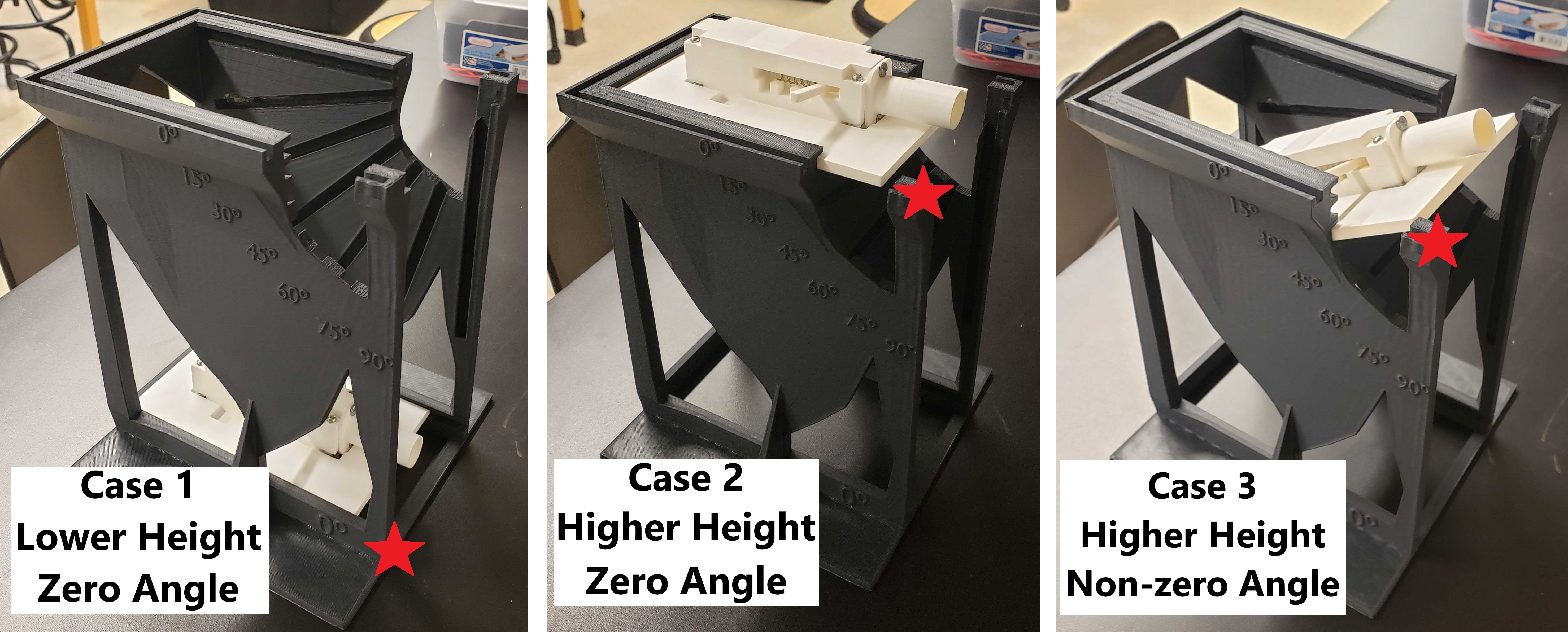
Figure 1:Stars denote projectile height. Left) Position of launcher for lower height in Case 1. Right) Position of launcher for higher height in Case 2. Right) Position of launcher for angled launches in Case 3 where the ball’s initial position is at the same higher height position.

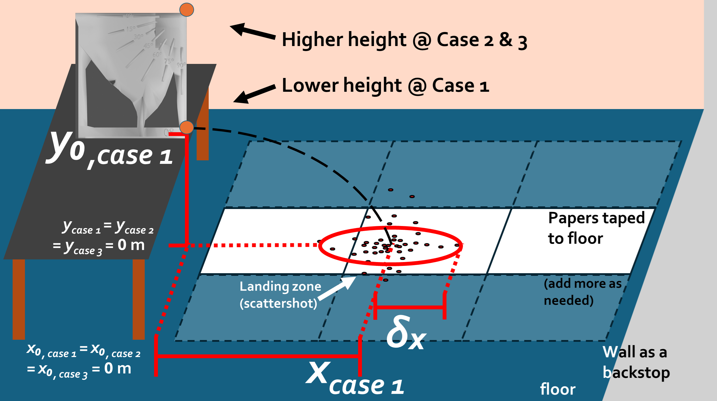
Figure 2:Example of Case 1 data aquisition.

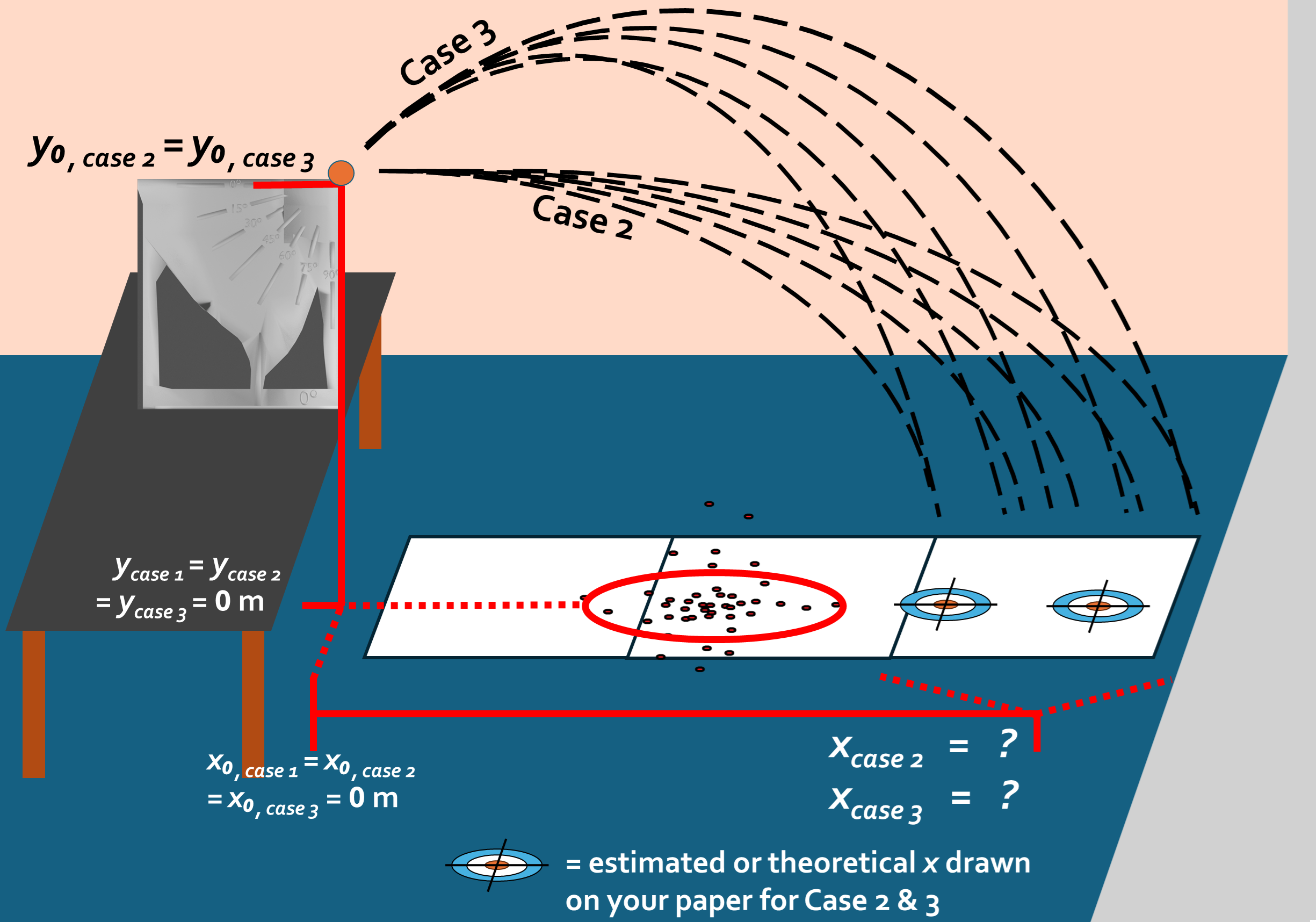
Figure 3:Example of Case 2 and 3 estimation and data aquisition.

○ Zero-Angle Trajectories (Background for Cases 1 & 2)¶

The distance traveled in the in the $x$ direction $\Delta x$ will be measured from the center of the ball in the uncocked position (initial position $x_0$ ) to the average landing position on the floor (final position $x$ ) after the given number of trials. Note: $\Delta x = x - x_0$ , however since initial position $x_0 = 0\,\text{m}$ for all cases throughout the lab today, $\Delta x = x$ .

The ball will mark up white printer paper with black carbon paper; we will note each landing point (e.g. with colored marker to ignore accidental carbon marks). We will then circle this scatter shot and estimate the average position of all trials from the given case, and then measure the distance with 1 and 2 meter sticks to determine final horizontal position $x$ .

After investigating how far the ball travels in the $x$ direction from a given height in Case 1, we can determine characteristics about the launcher-and-ball system to estimate how far in the $x$ direction we may expect the ball to travel when launched from a different initial height and/or angle in Cases 2 and 3.

To estimate how far the ball will travel horizontally in Case 2 where we move the launcher to the higher 0° slot (~19 -- 21 cm higher), we can use (5) to determine $x_{\text{case 2 theoretical}}$ . However, to do so, we will need to know:

for how long ( $t_{\text{case 2}}$ ) and
how fast ( $v_{0x\text{,case 2}}$ ) it will be moving

since distance traveled = speed $\times$ time.

To determine $v_{0x\text{,case 2}}$ , we can realize the balls are launched at a zero angle with respect to the floor, similar to that of Case 1. Therefore $v_{0x\text{,case 2}} = v_{0x\text{,case 1}}$ . Thus we can use our data from Case 1 to determine $v_{0x\text{,case 1}}$ . Since the total velocity for Case 1 is solely in the $x$ direction, we can also call $v_{0x\text{,case 1}}$ the launcher’s exit velocity $v_{\text{0,exit}}$ . Therefore for today, $v_{0x\text{,case 2}} = v_{0x\text{,case 1}} = v_{\text{0,exit}}$ .

Before we can solve for the exit velocity from Case 1 with (5), we need to know for how long the ball was in the air. If we call the ball’s final height on the floor $y$ , and we measure the initial height $y_{0}$ of the ball, we can use the height difference ( $\Delta y = y - y_0$ ) to determine the time $t$ it took to fall to the floor in the $y$ direction due solely to gravity $g$ . Rearranging (7) to solve for $t_{\text{case 1}}$ , and knowing that the ball starts at rest in the $y$ direction $\text{(}\,v_{0y{\text{,case 1}}} = 0\,\text{m/s}\,\text{)}$ and treating the floor as $y_{\text{case 1}} = 0\,\text{m}$ :

y = y_{0} + v_{0y}t - \frac{1}{2}gt^{2}~~~~~\Rightarrow~~~~~0 = y_{0} + 0 - \frac{1}{2}gt^{2}~~~~~\Rightarrow~~~~~\sqrt{\frac{2y_{0{\text{,case 1}}}}{g}} = t_{\text{case 1}}

(10)

Now that we know the time $t_{\text{case 1}}$ , and treating the uncocked position as $x_{0{\text{,case 1}}} = 0\,\text{m}$ , we can use (5) to determine the initial horizontal velocity $v_{0x\text{,case 1}}$ when released. Reminder, since the total velocity for the zero-angle launch was solely in the $x$ direction, we are calling this the launcher’s exit velocity $v_{\text{0,exit}}$ for the rest of the lab:

x = x_{0} + v_{0x}t~~~~~\Rightarrow~~~~~x = 0 + v_{0x}t~~~~~\Rightarrow~~~~~\frac{x_{\text{case 1}}}{t_{\text{case 1}}} = v_{0x{\text{,case 1}}} = v_{\text{0,exit}}

(11)

Now that we know $v_{0x\text{,case 2}} = v_{\text{0,exit}}$ at this higher height of Case 2, we focus on $t_{\text{case 2}}$ . Similar to before, we can solve for the time by measuring $y_{0\text{,case 2}}$ and plugging it into (10):

\sqrt{\frac{2y_{0\text{,case 2}}}{g}} = t_{\text{case 2}}

(12)

This leads us back to (5) where we want to solve for $x_{\text{case 2 theoretical}}$ . Using the time $t_{\text{case 2}}$ and by saying $x_{0\text{,case 2}} = 0\,\text{m}$ in the uncocked position, we find:

x = 0 + v_{x}t~~~~~\Rightarrow~~~~~x_{\text{case 2 theoretical}} = v_{\text{0,exit}}t_{\text{case 2}}

(13)

We will then launch the ball at Case 2’s height and see how accurate we estimated $x_{\text{case 2 theoretical}}$ . The experimentally determined $x_{\text{case 2 experimental}}$ will be measured in the same way as in Case 1 (circling and estimating the center of the scattershot).

○ Angled Trajectory (Background for Case 3)¶

The third case of this experiment is similar to Case 2 in that we are staying at the higher height, but now investigating angled trajectories and how far in the $x$ direction do they reach? The large, launcher holder is designed to hold the ball at rest (uncocked) in the same position (both horizontal and height) regardless of angle, so you can treat $y_{0\text{,case 3}} = y_{0\text{,case 2}}$ as your value for the ball’s initial height and $x_{0\text{,case 3}} = x_{0\text{,case 2}}$ for the ball’s initial horizontal position (see Figure 1 right).

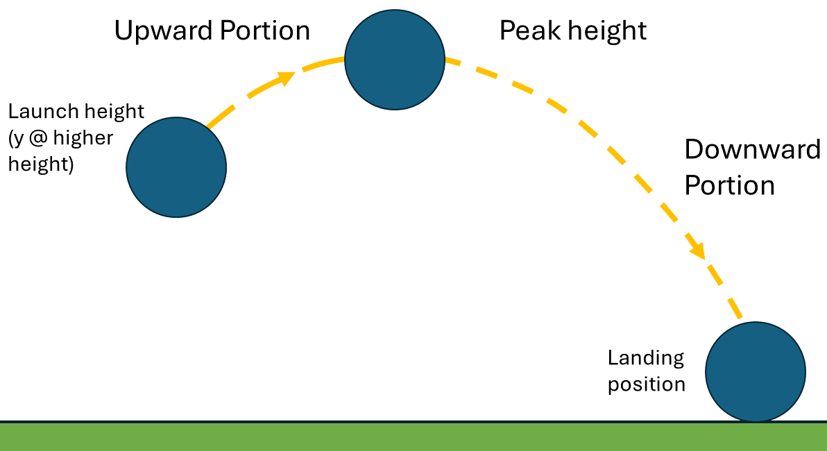
Figure 4:Example of the upward and downward portions you’ll analyze in Experiment 3 for an angled launch.

By launching at an upward angle $\theta$ (see Figure 4), we are now giving some of the initial velocity to both $x$ and $y$ directions. Once again, as there is no acceleration in the $x$ direction, we will ultimately use (5) to determine $x_{{\text{case 3,theoretical}}}$ . However, we need to know both $v_{0x\text{,case 3}}$ and $t_{\text{case 3}}$ . The velocity will merely be the horizontal component of the exit velocity determined in the previous cases:

v_{0x\text{,case 3}} = v_{\text{0,exit}}\cos{\theta}

(14)

To solve for the time, we can characterize motion in the $y$ direction to determine for how long the ball is in the air. One way to solve for the total travel time is via the quadratic equation with (7) (not shown here). An alternative method to find the total time can be conducted by breaking the trajectory into parts (i.e. $t_{\text{case 3}}~=~t_{\text{up}}~+~t_{\text{down}}$ as depicted in Figure 4) where $t_{\text{up}}$ is the time for upward travel from launch to the peak height, and $t_{\text{down}}$ is the time for downward travel to the floor from that peak height.

UPWARD PORTION $t_{\text{up}}$ ) Starting with (6), we know the initial velocity in the $y$ direction is the vertical portion of the exit velocity, $v_0 = v_{0y\text{,case 3 up}} = v_{\text{0,exit}}\sin{\theta}$ . At the peak of the trajectory, the ball goes to rest in the vertical direction such that the final velocity is $v_{y} = v_{y\text{,case 3 up}} = 0\,\text{m/s}$ , thus:

v_{y\text{,case 3 up}} = v_{0y\text{,case 3 up}} - gt_{\text{up}}~~~~~\Rightarrow~~~~~0 = v_{\text{0,exit}}\sin{\theta} - gt_{\text{up}}

(15)

leads to

\frac{v_{\text{0,exit}}\sin{\theta}}{g} = t_{\text{up}}

(16)

DOWNWARD PORTION $t_{\text{down}}$ ) For the downward travel, we can use (7) to determine the time $t_{\text{down}}$ it took to fall from the peak $y_{\text{0,case 3 down}}$ to the floor $y_{\text{case 3 down}}$ . To do this, we need to determine the initial velocity, initial height, and final height.

As mentioned in the upward portion, we know the velocity at the peak of the trajectory in the vertical direction is zero, therefore the downward portion’s initial velocity $v_{0y\text{,case 3 down}} = v_{y\text{,case 3 up}} = 0\,\text{m/s}$ . Then, as in previous cases, we also know the final height at the floor is $y_{\text{case 3 down}} = 0\,\text{m}$ .

To determine the initial height for the downward portion, we can realize this equals our final height from the upward portion (i.e. peak height $y_{\text{peak}} = y_{\text{0,case 3 down}} = y_{\text{case 3 up}}$ ). We can then use (7) to solve for the final peak height using values regarding the upward portion. We already know our measured initial launch height $y_{0\text{,case 3}}$ as noted from earlier measurements, and the initial velocity in the $y$ direction $v_{0y\text{,case 3 up}}$ and the time of the upward travel $t_{\text{up}}$ as used in (16). Plugging this all in to (7), we find the peak height to be:

y_{\text{peak}} = y_{0\text{,case 3}} + v_{\text{0,exit}}\sin{(\theta)}t_{\text{up}} - \frac{1}{2}gt_{\text{up}}^{2}

(17)

Now that we know $y_{\text{peak}}$ , we can use (7) also to solve for $t_{down}$ . Plugging in variables and substituting the zero floor height and zero initial vertical velocity:

y_{\text{case 3 down}} = y_{\text{peak}} + v_{0y\text{,case 3 down}}t_{\text{down}} - \frac{1}{2}gt_{\text{down}}^{2}~~~~~\Rightarrow~~~~~0 = y_{\text{peak}} + 0 - \frac{1}{2}gt_{\text{down}}^{2}

(18)

we subsequently get:

\sqrt{\frac{2y_{\text{peak}}}{g}} = t_{\text{down}}

(19)

HORIZONTAL DISTANCE) Finally, we have the total time $t_{\text{case 3}}~=~t_{\text{up}}~+~t_{\text{down}}$ from (16) and (19) as well as the initial velocity $v_{0x\text{,case 3}}$ from (14). Plugging into (5) to determine the theoretical distance $x_{\text{case 3 theoretical}}$ the ball with travel in the $x$ direction for any given non-zero angle $\theta$ :

x_{\text{case 3 theoretical}} = v_{\text{0,exit}}\cos{(\theta)}t_{\text{case 3}}

(20)

Experimental Procedure¶

● Procedure Preview¶

OVERVIEW

Investigate projectile motion in two-dimensions.
Conduct 3 cases as listed in Table 1. If time allows, the instructor may opt for additional angled cases.:
- Case 1: Zero-angle launches at a lower height. Characterize the trajectory and exit velocity from the marble launcher.
- Case 2: Zero-angle launches at a higher height. Calculate the theoretical trajectory (distance $x$ ); place a bullseye at your expected location and compare your experimental landing scattershot to the theoretical distance.
- Case 3: Angled launches ( $45^\circ$ ) at the same higher height. Calculate the theoretical trajectory (distance $x$ ); place a bullseye at your expected location and compare your experimental landing scattershot to the theoretical distance.
Conduct 40 -- 45 launches (trials) depending on group size for one overall measured data point for each case; estimate the experimental landing scattershot by circling your carbon-paper dots and estimating the center of the scattershot.

Table 1:Three Primary Experimental Cases with Four Extended Cases

Case	Height	Angle
1	Lower	$0^\circ$
2	Higher	$0^\circ$
3	Higher	$45^\circ$
Additional	Higher	$15^\circ$ , $30^\circ$ , $60^\circ$ , $75^\circ$

● Demo Video: Procedure for Simple Projectle Motion¶

Overview of Experimental Procedure for the Simple Projectile Motion lab. Notes: All launchers now use the orange balls.

● Case 1 --- Zero-angle Launch¶

Create a data table for Case 1 including but not limited to:
- Common data section with the accepted value of $g$ .
- Section containing:
  - the ball initial height $y_{0}$
  - the ball height’s estimated uncertainty $\delta y_{0}$
  - experimental overall distance $x$
  - experimental distance estimated uncertainty $\delta x$ based on the radius of the circle/ellipse you draw around the scattershot of all launches for case
- Additional sections for derived time of the trajectory $t$ and initial velocity $v_{\text{0,exit}}$ .
Place the marble launcher in the holder in the lower $0°$ slot (uncocked to represent where the ball will be once the piston is no longer accelerating the ball up to speed, and the ball is released).
Measure the height the ball will fall (as seen in Figure 2); place the ball into the launcher as the initial height $y_{0}$ is measured from the bottom of the ball to the floor (though the bottom of the inside of the barrel can also be used as the bottom of the ball location if that is easier to measure). Ensure the ruler you use has the zero meter end on the floor. Use a plumb bob to find and note the ball’s initial position on the floor.
Conduct a few test launches by pulling the piston back to the denoted notch for your launcher. Take mental note of where the ball is generally landing and ensure it’s generally consistent.
Which Loaded Piston Position?
Only pull piston back to slot denoted by arrows on the launcher itself.
Hold Launcher Plate
To help prevent the launcher from falling to the floor and breaking, please hold on to the rectangular plate that holds the launcher.
Push, don’t smack. Use release bar, not finger.
- Ensure the ball is resting against the piston such that the piston will push rather than hit the ball out of the launcher.
- Ensure you use the release bar, and not your finger, to quickly release the piston.
- Before continuing, try some test launches with the ball not resting against the piston. Notice the greater inconsistency.
- Before continuing, try releasing the launcher with just your finger instead of the release bar. Notice the greater inconsistency.
Get some pieces of white printer paper and tape them in the approximate landing zone, and place pieces of carbon paper on top (no need to tape that one since you’ll be moving it between trials) so the ball can mark up the white paper when it lands. Materials available at the table towards the middle of the room. Use this same set of paper throughout all cases.
Reminder: Share supplies
Please do not take the tape away from the table as everyone will need it, thanks
Conduct 40 -- 45 launches onto the paper/carbon paper. Make sure the launcher plate is the whole way into the slot to ensure a consistent starting position. Between each launch, move aside the carbon paper and mark each dot with a marker or something else that makes it apparent which dots are your data points for this case. Additional markers should be available on the table towards the middle of the room.
Reminder: Take turns
- Groups of 2 students, each student will conduct 20 launches for a total 40/case.
- Groups of 3 students, each student will conduct 15 launches for a total 45/case.
Hold Launcher Plate - Safety and Consistency
- To help prevent the launcher from falling to the floor and breaking, please hold on to the rectangular plate that holds the launcher.
- Holding the plate the whole way back each time can also provide additional consistency to your launches.
Draw a rough circle/ellipse surrounding the scattershot of all launches across all group members for the current case. Flashlights are available at the table towards the middle of the room that could asist in drawing your circle/ellipse. (e.g. Figure 5) Something to consider when determining how large your circle/ellipse should be: remember that we’ve used the standard deviation (the spread of the data relative to the mean) as a stand-in for uncertainty in previous labs. The standard deviation typically includes about two-thirds of the data. Therefore, for use in the following steps, you can estimate your average horizontal distance and uncertainty by drawing a circle/ellipse that encompasses roughly two-thirds of your data, centered around the densest region of your scattershot. Mark the center of your circle/ellipse with a cross hair to represent your average horizontal distance.
Measure the single value for the experimental distance $x$ from the center of the ball at rest in the barrel (uncocked) to the cross hair center that you drew in your scatter shot on the floor. To translate the initial location of the ball in the barrel to the floor, use a plumb bob to make a straight line down to the floor for $x_0\text{,}$ from which you can more easily measure final distance $x$ .
From your circle around your scattershot, estimate and measure your uncertainty in horizontal distance $\delta x$ , effectively the radius of your circle/ellipse. (if coming from Case 2, return to step 15; if Case 3, return to step 26)
Future Photo of Experimental Data
At the end of Case 3, you will take a photo of all of your data to include in your spreadsheet / data submission (example in Figure 5). Do not dispose of your paper or untape it from the floor; you will continue to use it in future cases. Add paper as needed for additional cases.

● Case 2 --- Zero-angle Launch at a Higher Height¶

Create additional data section for Case 2 including but not limited to:
- Height of the ball at the higher $0°$ slot height $y_{0\text{,case 2}}$
- Time of the trajectory from a higher height $t_{\text{case 2}}$
- Theoretical distance $x_{\text{case 2, theoretical}}$
- Experimentally measured distance $x_{\text{case 2, experimental}}$
- Estimated uncertainty in the experimental distance $\delta x_{\text{case 2, experimental}}$ (essentially ± the radius of the circle drawn around your scattershot)
- Difference (magnitude) between the theoretical and experimental $x$ distances
Move the marble launcher to the higher $0°$ slot and remeasure the initial height $y_{0\text{,case 2}}$ (see Figure 3). Use a plumb bob to ensure you measure vertically.
Now, calculate the theoretical distance $x_{\text{case 2, theoretical}}$ using (10) -- (13).
Add paper as needed. Before any launches from the higher height, draw a bullseye at the theoretical distance you expect the balls at the higher height to land to visually see how close we get. You can draw both a cross hair for the distance and estimate how big the scatter will be (to discuss later in Post-Lab Submission --- Interpretation of Results). See example in Figure 3.
Conduct a few test launches by pulling the piston to the same notch you’ve been using in previous case(s) to ensure you have paper coverage for the landing zone. Additionally, by using the same notch, you will also be able to use the same exit velocity as previously determined for the launcher. Add paper as needed.
If need be, tape additional paper in the location from the test launches, while still including paper from previous case(s). Place (no tape needed) a piece of carbon paper on top (no need to tape that one) so the ball can mark up the paper when it lands.
On the same set of white paper on the floor as you retrieved in step 5, repeat steps 6 to 9 to experimentally determine the horizontal distance and its uncertainty when launched from the higher height (i.e. $x_{\text{case 2, experimental}}$ and $\delta x_{\text{case 2, experimental}}$ ).
Calculate the difference (magnitude, not percent) between your theoretical and experimental values of $x_{\text{case 2}}$ .
Discussion Point
- To be discussed further in Post-Lab Submission --- Interpretation of Results.
- Does your experimental distance from the higher height agree with what you expected from your theoretical calculation? In other words, does $x_{\text{case 2, experimental}} \pm \delta x_{\text{case 2, experimental}}$ overlap with $x_{\text{case 2, theoretical}}$ (i.e. does your uncertainty cover the difference between the experimental and theoretical values?)?

● Case 3 --- Angled Trajectory at a Higher Height¶

Create additional data section for Case 3 including but not limited to:
- Common data section with the accepted value of $g$ and any values you will need from previous cases to determine the theoretical horizontal distance at a given angled launch ((14) to (20)).
- Additional sections for:
  - Theoretical distance $x_{\text{case 3, theoretical}}$
  - Experimentally measured distance $x_{\text{case 3, experimental}}$
  - Estimated uncertainty in the experimental distance $\delta x_{\text{case 3, experimental}}$ (essentially ± the radius of the circle drawn around your scattershot)
  - Difference (magnitude) between the theoretical and experimental $x$ distances
Place the marble launcher in the holder in the $45^\circ$ slot (see Figure 3).
Use your previously measured $y_{0\text{,case 2}}$ as the height the ball will fall for any angled launches (e.g. $y_{0\text{,case 2}} = y_{0\text{,case 3}}$ ) as the large holder is designed to release the ball from the same position regardless of angle.
Calculate the theoretical distance $x_{\text{case 3, theoretical}}$ using (14) to (20).
Before any launches from the higher height for the non-zero angle, draw a bullseye at the theoretical distance you expect the balls to land to visually see how close we get. You can draw both a cross hair for the distance and estimate how big the scatter will be. Add paper as needed.
Conduct a few test launches by pulling the piston to the same notch you’ve been using in previous case(s) to ensure you have paper coverage for the landing zone. Additionally, by using the same notch, you will also be able to use the same exit velocity as previously determined for the launcher.
If need be, tape additional paper in the location from the test launches, while still including paper from previous case(s). Place (no tape needed) a piece of carbon paper on top (no need to tape that one) so the ball can mark up the paper when it lands.
On the same set of white paper on the floor, repeat steps 6 to 9 to experimentally determine the horizontal distance and its uncertainty when angle-launched from the higher height (i.e. $x_{\text{case 3, experimental}}$ and $\delta x_{\text{case 3, experimental}}$ ).
Calculate the difference (magnitude, not percent) between your theoretical and experimental values of $x_{\text{case 3}}$ .
Discussion Point
- To be discussed further in Post-Lab Submission --- Interpretation of Results.
- Does your experimental distance from an angled launch at the higher height agree with what you expected from your theoretical calculation? In other words, does $x_{\text{case 3, experimental}} \pm \delta x_{\text{case 3, experimental}}$ overlap with $x_{\text{case 3, theoretical}}$ (i.e. does your uncertainty cover the difference between the experimental and theoretical values?)?
If there are additional angles assigned, move the marble launcher to the respective angle and repeat steps 6 to 9 as needed, as well as step 27.
TAKE A PHOTO OF ALL YOUR DATA (paper with all your marble impacts measured and labeled across all cases).
Photo of Experimental Data
Take a photo to include in your Excel datasheet / spreadsheet submission.
Return carbon paper and other supplies
If your carbon paper is still intact, please return it to the pile on the table towards the middle of the room for use in future labs.

Post-Lab Submission --- Interpretation of Results¶

● Finalized Spreadsheets¶

Make sure to submit your finalized data table (Excel sheet).
- Please include relevant plot(s) including:
  - A photo of your experimental landing-zone data papers (while still taped to floor to show distribution).

● Post-lab Writeup¶

In a paragraph, summarize your error analysis. Be both qualitative and quantitative. Argue your conclusions with your data values.
- What is the precision of your equipment?
- What are possible systematic errors for today’s experiments?
- What sources of error may contribute to larger scatter from each case (i.e. size of your estimated ellipse radius that represented $\delta x$ )?
- How does your estimated uncertainty for Case 1 affect your theoretical distances for Cases 2 & 3, larger or smaller? Try, in your spreadsheet, changing your $x_{\text{case 1}}$ by its uncertainty, i.e. $x_{\text{case 1}} + \delta x_{\text{case 1}}$ . How much bigger or smaller does your $x_{\text{case 2, theoretical}}$ and $x_{\text{case 3, theoretical}}$ become?
- Cases 2 & 3:
  - What uncertainties or sources of error might make the difference between your theoretical and experimental horizontal distances larger or smaller?
In a paragraph, summarize the results you have determined in each case, i.e. $x_{\text{experimental}} \pm \delta x_{\text{experimental}}$ ... and answer the following questions (longer does not mean better) while arguing your conclusions with your data values:
- What type of system do the kinematic equations represent?
- Cases 1 & 2:
  - What were your results for the horizontally-launched trajectories at the initial lower height and then higher height? Do your results $x_{\text{case 2, experimental}} \pm \delta x_{\text{case 2, experimental}}$ overlap with $x_{\text{case 2, theoretical}}$ ? If not, what may be a physical reason why?
- Case 3:
  - What were your results for the trajectories from a non-zero angle(s) at the higher height? Do your results overlap with your theoretical value? Another way to think about it, does your uncertainty cover the magnitude of the difference between your experimental and theoretical values? If not, what may be a physical reason why?
- Were your bullseye targets (estimation) accurate to the experimental results; any bias towards being an over- or under-estimate? Back up your answer with your results.

The Whiteboard¶

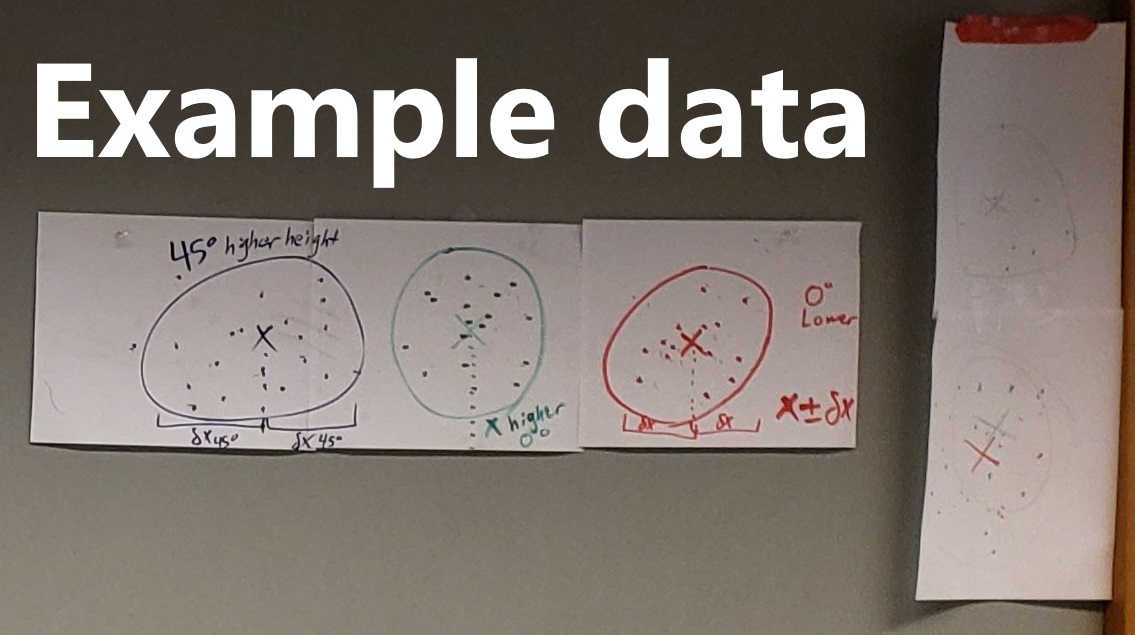
Figure 5:Examples of what experimental data may look like including uncertainty estimations.