Conservation of Energy with Glider on Tilted Air Track
Background
● Background Overview
Energy cannot be created nor destroyed. All that can really happen is a change in its form. We shall consider the conservation of mechanical energy, in particular, the sum of the kinetic energy and potential energy of a mass. The kinetic energy is due to the motion of the mass and the potential energy is due to the relative position of the mass in the earth’s gravitational field. This total mechanical energy can only change if nonconservative forces are acting on any part of the system. We will examine the exchange of kinetic and potential energy and the conservation of mechanical energy under the presumption of no nonconservative forces acting. If the mechanical energy is not conserved we will attempt to determine potential sources of nonconservative work being done that would change the mechanical energy.
The work done by a force acting on a mass is the magnitude of the force acting in the direction of motion times the distance the mass moves. Work is only done when the mass moves. (In other words, you can push as hard as you like on a brick wall, but if the wall doesn’t move, you didn’t do any work!) Assume for the moment that we have a mass moving on a frictionless, horizontal surface. Assume a force acts on the mass from the position to as illustrated in Figure 1. At position it is moving with a velocity and at the velocity is .
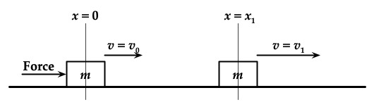
Figure 1:Explanation of the variables needed to calculate the amount of work done on a mass
The work done by the force is . Using Newton’s second law it can easily be shown that the work done by the force changes a quantity we call the kinetic energy, . Using the example illustrated in Figure 1,
In this case, the force is acting in the direction of the motion and thereby increases the kinetic energy. If the force were acting in the direction opposite to the motion, then the kinetic energy would be decreased. If friction were present, it would act in the direction opposite to the direction of motion and thereby reduce the kinetic energy. In this simple analysis, we have made no assumption as to the nature of the force.
A force like friction is a non-conservative force. The work done by it not only depends upon the path the mass takes but is also not completely recoverable. However, the work done on a mass by a conservative force can be completely returned to the mass as mechanical energy. Thus work done by a conservative force can be represented by a potential energy function and depends only on the end points of the process. The gravitational force is a conservative force and is assumed constant in the vicinity of the surface of the earth. The potential energy function is merely the work done by gravity on the way up or the way down and is equal to the gravitational force (the weight ) times the change in height, . The gravitational potential energy, , is given by
The work done by this conservative force, like all conservative forces, only depends on the end-points of the path. The gravitational potential energy is a relative quantity, i.e., it is a change in energy because of a change in elevation. Thus we can choose a zero level arbitrarily.
If there are no non-conservative forces acting, then a mass moving only under the influence of gravity merely exchanges its kinetic and potential energy while the total energy remains constant. For a mass stationary at some height, , above the ground, all of its energy is potential energy of value with respect to the ground. As the mass begins to fall under the influence of gravity, it loses and gains . When it reaches the ground, the is zero with respect to the ground and the is a maximum, equal to the original at the top. If the mass were a roller coaster, the coaster could climb back up to its original height where all the energy would be at which point it would momentarily stop, i.e., no . This assumes that neither friction nor any other nonconservative force is acting. In general, we have
where is the work done by non-conservative forces. If there are no non-conservative forces acting, then
In this experiment, we will use an air track to provide a nearly frictionless surface. The track will be tilted at a measurable angle. A glider will be released from rest at the top of the track and allowed to slide down and collide with a spring at the bottom. If the force of the spring on the glider is conservative, then the kinetic energy of the glider at the bottom is converted to potential energy in the compressed spring. This potential energy is given back to the glider in the form of kinetic energy as the spring expands. The glider bounces off and goes back up the track to its original height where the energy is again all . If no energy is lost in the collision at the bottom, we say that the collision is completely elastic, implying that the forces involved in the collision are conservative. After the collision, the glider will rebound up the track. Getting back to its original height therefore implies no mechanical energy is lost during the entire path. If it does not, we have to look for an energy loss mechanism and some non-conservative forces acting.
The change in height from the top to the bottom is measured allowing the change in to be calculated. We will set the zero level for the potential energy at the bottom of track, at the position, , in Figure 2.
A measurement of the transit time from the top to the bottom will allow the calculation of the velocity at the bottom and therefore the at the bottom. Finally, measuring the maximum height achieved on the rebound will yield a second value of .
The at the bottom of the track can be determined by measuring the average velocity from the release point at the top, , to the collision point at the bottom, , and then using (4). From a measurement of the transit time from to , the velocity of the glider at the moment of collision at the bottom, , can be determined by using the definition of average velocity, , thus:
where the initial velocity, , is the distance traveled down the track, and is the transit time of travel.
Rearranging terms we have the velocity at the bottom in terms of measurable quantities
Using the definition of , the at the bottom is then
In order to calculate the potential energy, at any point, along the track we must determine the change in height between and . The potential energy at any position along the track is measured with respect to the collision point at the bottom, , which is arbitrarily assigned a value of zero potential energy. The is given by the weight of the glider, , times the change in vertical height.
Figure 2 is a simplified diagram of the inclined track. The distance is measured along the track by the scale attached to the side of the track. The change in elevation, , of any other point along the track can now be determined from the distance and the incline angle of track, . The incline of the track is produced by placing a spacer of known height under a leg at one end. With the height of the spacer and the distance between the legs, , the angle can be calculated (See Figure 3).
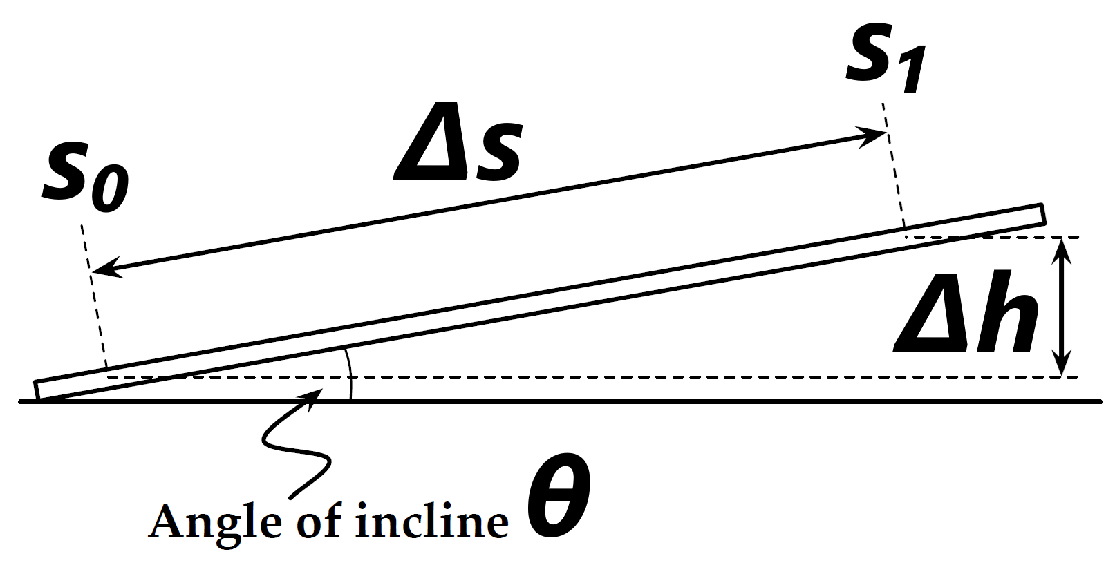
Figure 2:Schematic Drawing explaining the relationship between the track elevation and the distance for the Conservation of Energy experiment.
At , , therefore . Referring to our schematic of the experimental setup in Figure 3, we see or
therefore the potential energy, , at some position, , along the track is finally given by measurable quantities as
Experimental Procedure
● Procedure Preview
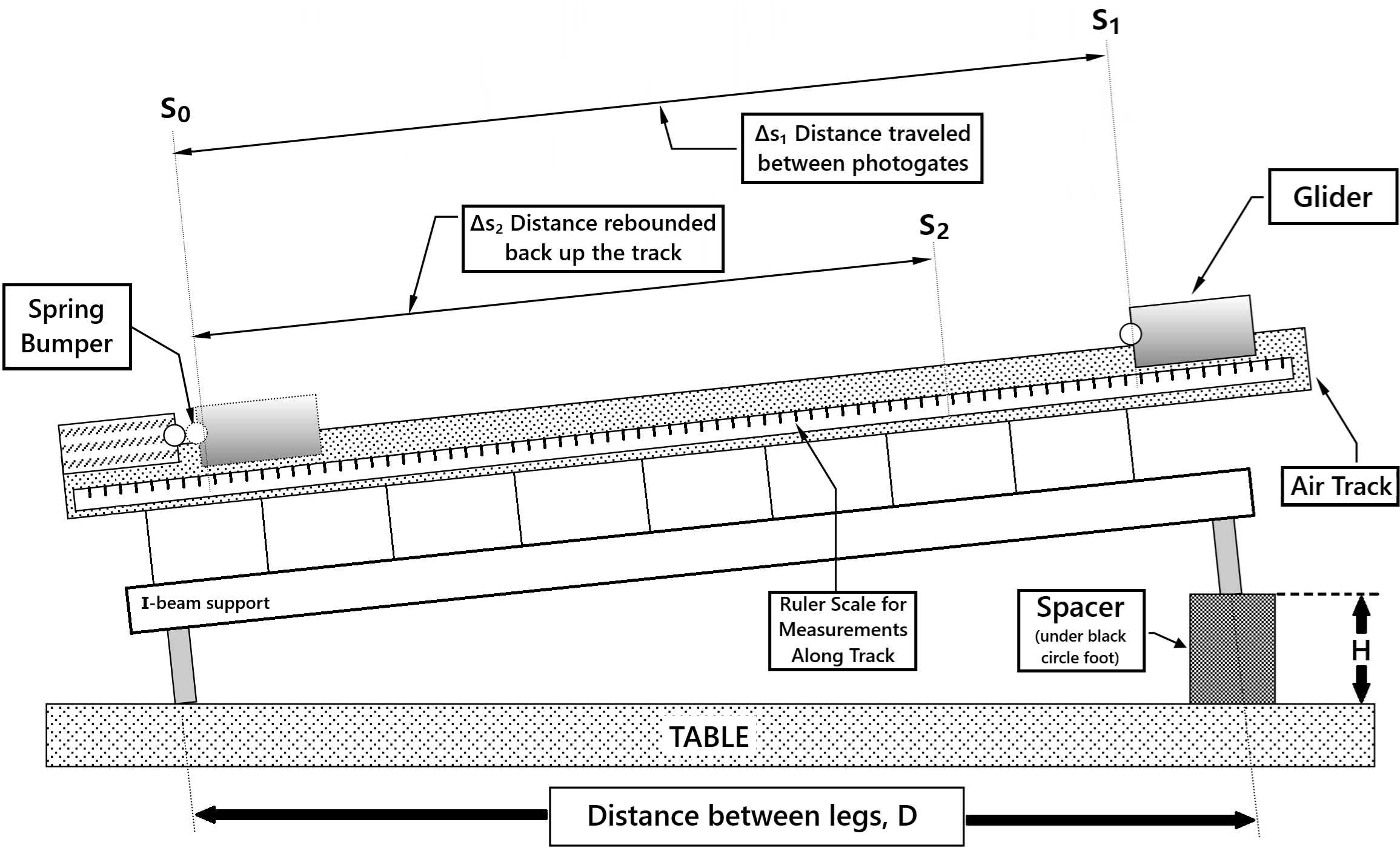
Figure 3:Experimental setup for the Conservation of Energy experiment.
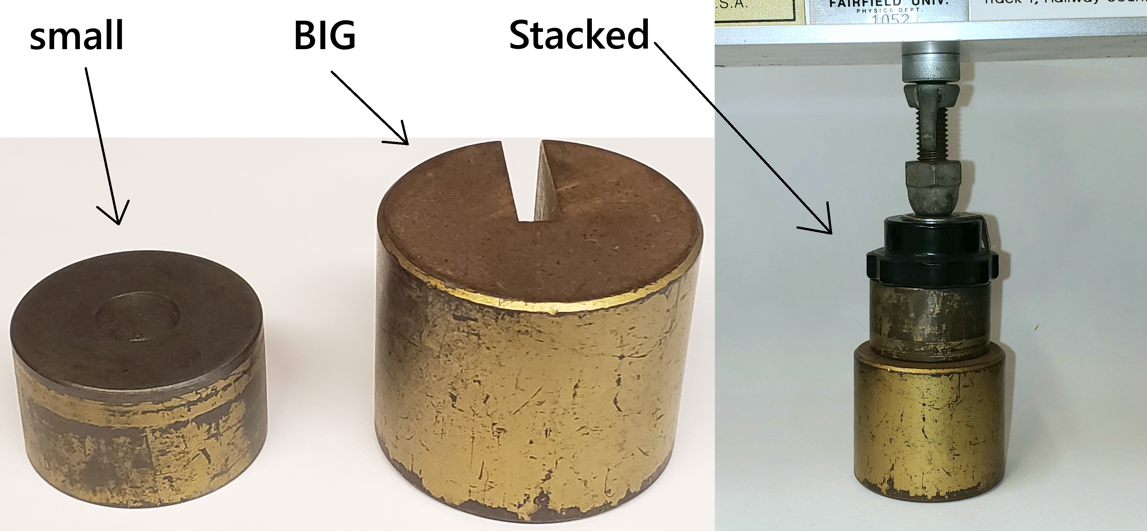
Figure 4:Example of small and large spacers used to incline the air track. The cases today will be the BIG and Stacked heights. Remember to put the black plastic footer on top of the spacers as shown in the stacked case.
● Preliminary Setup
Do not put a glider on the track without air flowing. If the air supply is not yet on, please remind the instructor.
Create a common data table including:
accepted value of of for Fairfield, CT
the masses of each of the gliders in kg
the distance between the legs of the air track in meter (m)
the heights of the two spacers (big slotted masses) in m
: starting point at the top
: stopping point at the bottom
: distance between the photogates that the glider travels down along the track
Measure and record the mass of both the big and small glider with the triple-beam-balance.
Level the airtrack. Without the spacer present and the air track resting directly on the tabletop (with the black circle feet), place one of the gliders on the track (somewhere between the photogates, center) and note any preferential drift of the glider. Adjust the height of the single leg (screw clockwise in or counter-clockwise out) until the air track is level, as indicated by no preferential drift. Check both orientations of the glider on the track to check if the car is asymmetric and has a significant preferential drift on an otherwise level track. If this occurs, make sure to note that for your discussion purposes.
Measure and record the distance . This is the center-to-center distance between the legs. 1 m and 2 m long meter sticks are available for this measurement, with additional meter sticks at the front wall of the room.
Measure and record the heights, , of each of the two spacers (big slotted masses) with the provided Vernier caliper. If you need a refresher on using Vernier calipers, see Reading the Vernier scale. Since we’ll be stacking the spacers for some of the cases today, include a stacked spacers value in your common data table for easier use of the height later.
Take a look at the gliders and determine a convenient point on the glider to use with the scale ( meter ruler) attached on the side of air track. It doesn’t matter what point on the glider you choose, only that you be consistent and use the same point for all determinations of distance along the track for that glider. A convenient point is the lower front or rear corner of the glider since it is a clear point on the glider that will overlap or be quite close to the length scale on the track itself (see Figure 5).
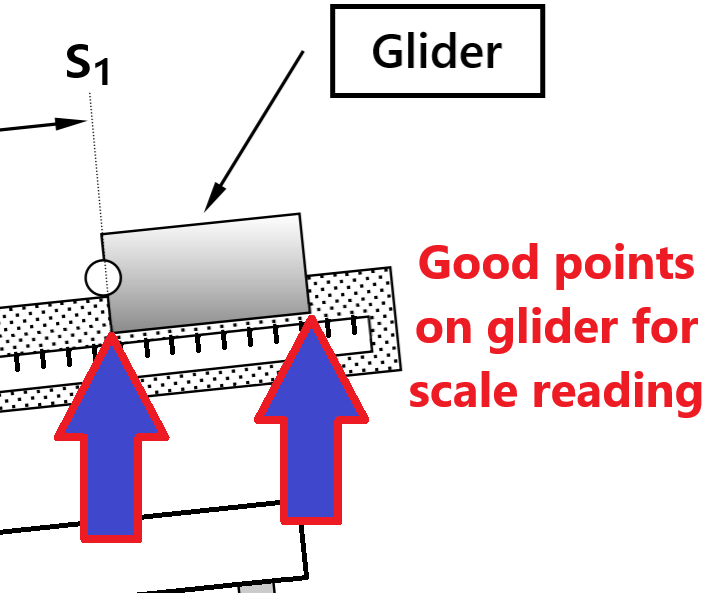
Figure 5:Suggested points on glider to read position on airtrack scale.
Determine and record the bottom photogate position at the bottom end of the track. Place the glider near the bottom of the track. Move it slowly as you approach the bottom photogate. Stop the glider at the exact location when the photogate’s red light comes on. Move the glider back and forth to confirm your scale reading. See ○ Demo Video: Photogate Positions for example method.
○ Demo Video: Photogate Positions
Determine photogate position on air track with glider.
Similarly, determine and record the starting photogate position at the top end of the track, then use those values to calculate and record . Place the glider near the top of the track. Move it slowly as you approach the top photogate. Stop the glider at the exact location when the photogate’s red light comes on. Move the glider back and forth to confirm your scale reading. Ensure your scale reading on the track was based on the same location of the glider as for your reading (i.e. Figure 5).
Four cases will be performed as listed in Table 1. For each of the four cases, perform the following steps listed in ● Experimental Data Collection and record the data appropriately in your spreadsheet. Note: We are not doing the small spacer by itself today.
● Experimental Data Collection
For each of the four cases, create a data table with enough rows for the number of trials you are doing along with average and standard deviations, and columns for each of the variables you will be measuring or deriving:
Trial number
Lab member’s initials
: start time at the top
: stop time at the bottom
: time of travel between the photogates
: The rebound position partway up the track
: Initial potential energy at top
: The speed at the bottom
: Kinetic energy at the bottom
: Final rebounded distance
: Final potential energy at the rebound position
: Percent change in mechanical energy during the first sequence of motion (top to bottom)
: Percent change in mechanical energy during the second sequence of motion (top to rebound)
Ensure and haven’t changed.
Raise the single leg side of the track by placing the case-relevant spacer under the black foot as seen in Figure 3 and Figure 4.
Before you take the recorded data in the next steps, take some practice runs. Your subsequent data will be much improved by your training! Review the following demo videos as well.
○ Demo Videos: Glider Release
Demonstration of glider release to minimize initial velocity.
○ Demo Video: Energy Conservation Across Single Trial
Demo video: Trial of Energy Conservation on the Airtracks. Note: This video predates the use of the timer in Capstone, so you will see an older style of timer.
Press record in Capstone to start the timer.
For each of the 6 trials per case, release the glider from rest at the position. Note the rebound position where the glider returns to rest after it rebounds up the track. Measure and record the start time and end time to determine transit time from the release at the top to bottom of the airtrack. Calculate the value of potential and kinetic energies, and discuss the conservation of energy throughout the experiment. To do so:
a. Position the glider so it is blocking the top photogate and the red light is on. Use the red glider-release mechanism to hold the glider in place. Shift the mechanism up or down the track as necessary to move and hold the glider just before the photogate beam such that the red light on the photogate just goes out.
b. Check the Capstone timer is ready, then release the glider by quickly flipping the glider release bar to minimize any additional push or pull on the glider to ensure its initial velocity is zero. (reminder, see ○ Demo Videos: Glider Release).
c. Allowing the glider to rebound off the bumper, record the rebound position . As the glider slows to a stop, capture the glider by gently pressing your finger near the lower edge of the glider just as it comes to a stop and then read off the scale. Use the same point on the glider to read that you used to read and (Figure 5).
d. Record the relevant and values in your spreadsheet. There is not a time for the rebound position. Calculate .
e. Calculate the relevant velocity, distance, and energies at the top starting point, the bottom of the track, and the ending rebound position (i.e. , , , , ) using (6), (7), (9).
f. Calculate , the percent change (10) in mechanical energy from the initial release point to the bottom photogate position (Note: If you change the Excel number format of this cell to
Percentagedo not multiply by 100 as Excel will do that for you).g. Calculate , the percent change (10) in mechanical energy from the initial release point to the final rebound point .
○ Averaged Results for Current Case
Calculate the average and standard deviations of your measured and experimentally determined values from to .
Repeat the previous steps in ● Experimental Data Collection for the next case as listed in Table 1. After you’ve completed all cases, move on to the next section summarizing your data from all cases.
● Summarized Results for Entire Lab
Create a summary table of the analysis with a section for each case including the averages (denoted by overbar) and standard deviations (denoted by sigma, ) of the following:
and
and
and
and
and
Post-Lab Submission --- Interpretation of Results
● Finalized Spreadsheets
Make sure to submit your finalized data table (Excel sheet).
● Post-lab Writeup
In a paragraph, summarize your error analysis. Be both qualitative and quantitative.
What is the precision of your equipment?
What are possible random errors for today’s experiment?
What are possible systematic errors for today’s experiments?
Answering using physics reasoning: How could one gain energy during the top-to-bottom sequence?
For today’s lab, assume that your calculated kinetic energies are their average +/- standard deviation values where the uncertanty comes from only the spread of the data. However, regarding the quantities of potential energy (at both top and rebound positions), consider for just one case:
Our measurable quantities (reminder (9)) and their estimated uncertainties (i.e. how confident you are in each of those values, rather than just your tools’ precision).
What are the effects of those measurement uncertainties on your determined potential energies? (e.g. how does affect )?
In a paragraph, summarize the results you have determined in each case. Consider:
Arguing your responses with your average values ± standard deviations:
Is kinetic plus potential energy conserved going from the top to the bottom?
Is kinetic plus potential energy conserved between the top and the rebound position?
Why is there a difference in energy conservation between the top-to-bottom sequence and top-to-bottom-to-rebound sequence? Explain using physical concepts and reasoning.
The Whiteboard