Fluid Physics with Archimedes’ & Bernoulli’s Principles
Background
● Background Overview
Matter most commonly exists as a solid, liquid, or gas; these states are known as the three common phases of matter. We will investigate liquids in today’s experiments. While solids are rigid with specific shapes and definite volumes where molecules are locked in position with their neighbors, liquids and gases are considered to be fluids because they are not rigid where the molecules are not locked in place and can therefore flow (i.e. move with respect to each other).
In today’s experiments, we seek to understand why objects float or sink in a liquid (water) using Archimedes Principle regarding fluid statics as well as how liquid flows using Bernoulli’s Principle regarding fluid dynamics.
● Archimedes’ Principle
Archimedes’ Principle states: “When an object is submerged in a fluid, the fluid exerts an upwards buoyant force equal to the weight of the fluid displaced by the object.”
As depth increases, pressure in a fluid increases. Therefore, for an object in a fluid, the upward force on the bottom of that object is greater than the downward force on top of that object (see pressure forces vs in Figure 1 left). There is a net upward force, or buoyant force, on any object in any fluid. If the buoyant force is greater than the object’s weight, the object will rise to the surface and float. If the buoyant force is less than the object’s weight, the object will sink (depicted in Figure 1 right-a with ). If the buoyant force equals the object’s weight, the object will remain suspended at that depth. As such, there is always a buoyant force acting on an object regardless of whether it floats, sinks, or remains suspended.
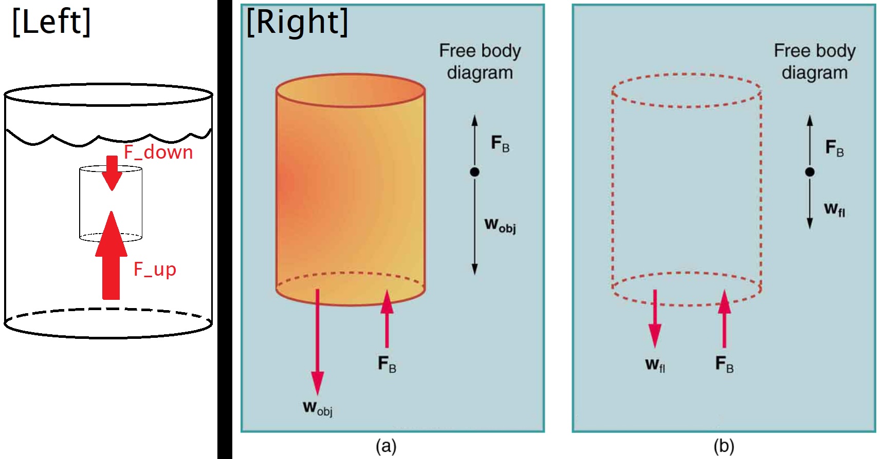
Figure 1:LEFT) Pressure due to the weight of a fluid increases with depth causing a greater upward force on the bottom of the object than the smaller downward force on the top of the object. ( and horizontal forces cancel.) RIGHT-a) An object submerged in a fluid experiences a buoyant force . If is greater than the weight of the object , the object will rise. If as depicted in a, the object will sink. RIGHT-b) If the object is removed, it is replaced by fluid having weight . Since this weight is supported by surrounding fluid, the buoyant force must equal the weight of the fluid displaced. That is, , a statement of Archimedes’ principle.
How could we determine the buoyancy force acting on the object within the fluid? It helps to describe this by removing the object (as in Figure 1 right-b). The volume of the space left behind is filled in by fluid having a weight . Since that fluid is supported by the surrounding fluid, that weight of the fluid (originally displaced by the object) is equal to the buoyancy force . This is Archimedes’ Principle --- The buoyant force on an object equals the weight of the fluid it displaces:
● Bernoulli’s Principle
Imagine fluid flowing through a channel of varying width (ex. of such a setup in Figure 2). As the cross-sectional area changes, the volumetric flow rate remains constant, but the velocity and pressure of the fluid vary.
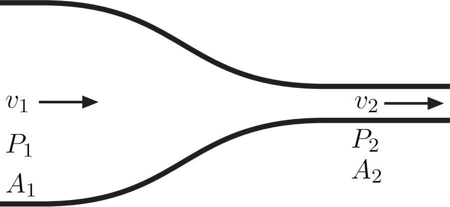
Figure 2:Example of a Venturi tube, where velocity , pressure , and cross-sectional area
An incompressible fluid of density flows through a pipe of varying diameter. As the cross-sectional area decreases from (large) to (small), the speed of the fluid increases from to . The flow rate, , of the fluid through the tube is related to the speed of the fluid () and the cross-sectional area of the pipe . The flow rate must be constant over the length of the pipe as everything that goes in one side comes out the other end. This relationship is known as the Continuity Equation which can be expressed as:
As the fluid travels from the wide part of the pipe to the constriction, the speed increases from to , and the pressure decreases from to . This drop in fluid pressure due to fluid speeding up as it flows through a constricted section of a pipe is known as the Venturi effect. This effect can be created with the use of a Venturi tube which allows an incompressible fluid to flow from a wider to narrower section with minimal turbulence.
Assuming the path an incompressible fluid takes is frictionless with no viscous forces, then the energy of the fluid is conserved. The fluid can be analyzed by the total work done on the fluid from the initial position to final position within the tube (total change in both kinetic and potential energy). The full derivation is in your lecture textbook, but for now, we arrive at Bernoulli’s Equation. For an incompressible, frictionless fluid, the combination of pressure and the sum of kinetic and potential energy densities is constant not only over time, but also along a streamline:
Note the similarities in (3) to our previous labs’ equations for kinetic and potential energies ( & ). Applying this to our Venturi tube of Figure 2:
However, since our tube will be horizontal, we can remove the height dependence and our pressure change is due only to the velocity change (noted by the Continuity Equation in (2)). Thus, our equation simplifies to Bernoulli’s Principle of fluid flow at a constant height:
Rearranged another way to determine the pressure at the constriction:
Experimental Procedure
● Demo Video: Procedure Summary
Demonstration video: The whole Fluids lab.
--- https://
● Archimedes’ Principle (First experiment)
○ Archimedes --- Preliminary Setup
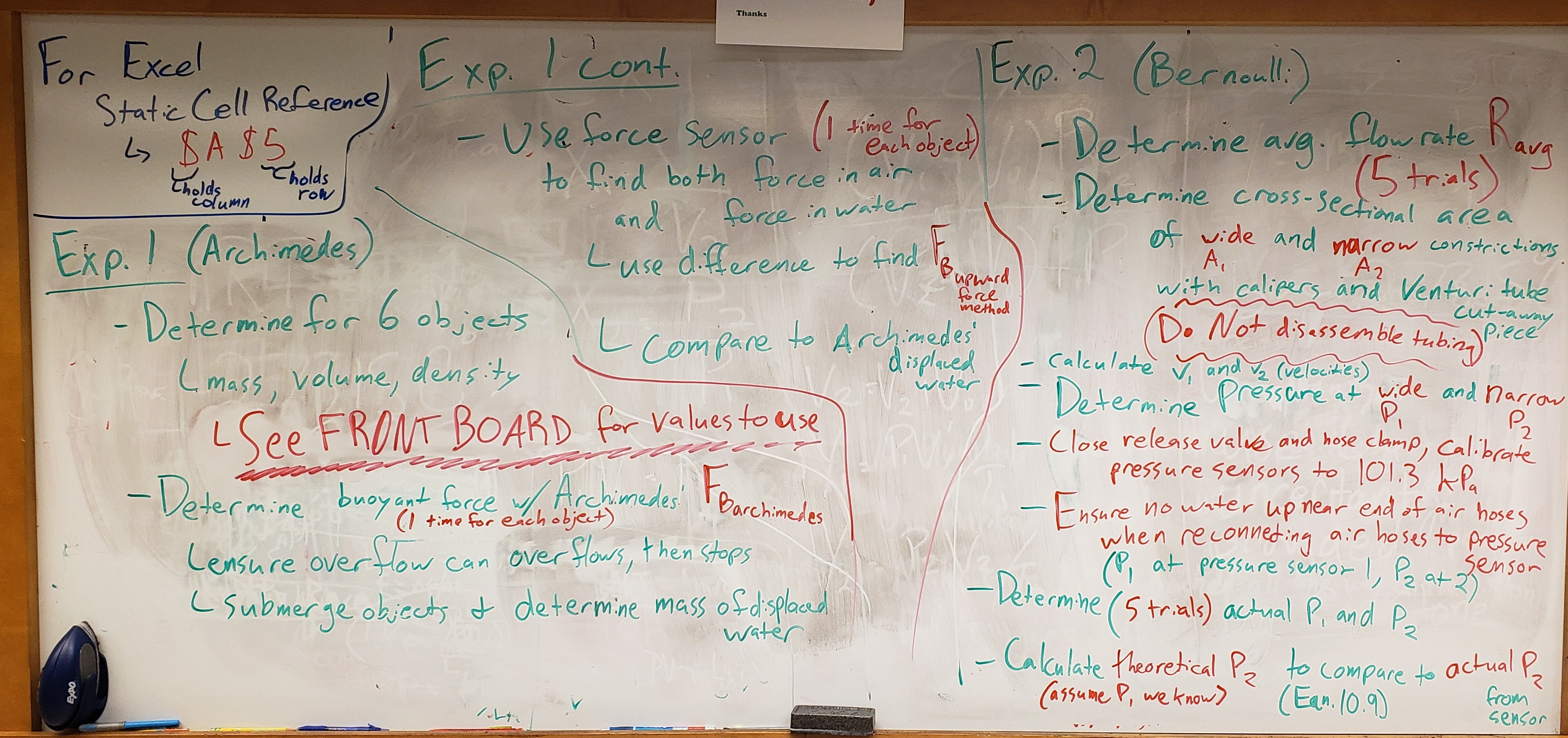
In this experiment, we will first determine the mass, volume, and density of 6 objects (see Figure 3). We will then determine the buoyant force acting on each object using Archimedes’ Principle by determining the weight of water each object displaces. Finally, we will determine the buoyant force by measuring the apparent weight of an object.
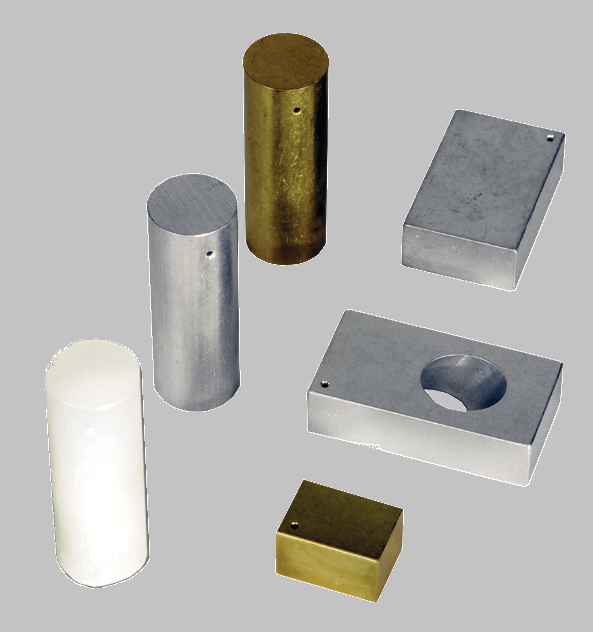
Figure 3:3 cylinders, 2 blocks, 1 irregular shape.
As a reminder, the density of an object depends on its mass and volume :
and the weight of an object is the downward force due to gravity:
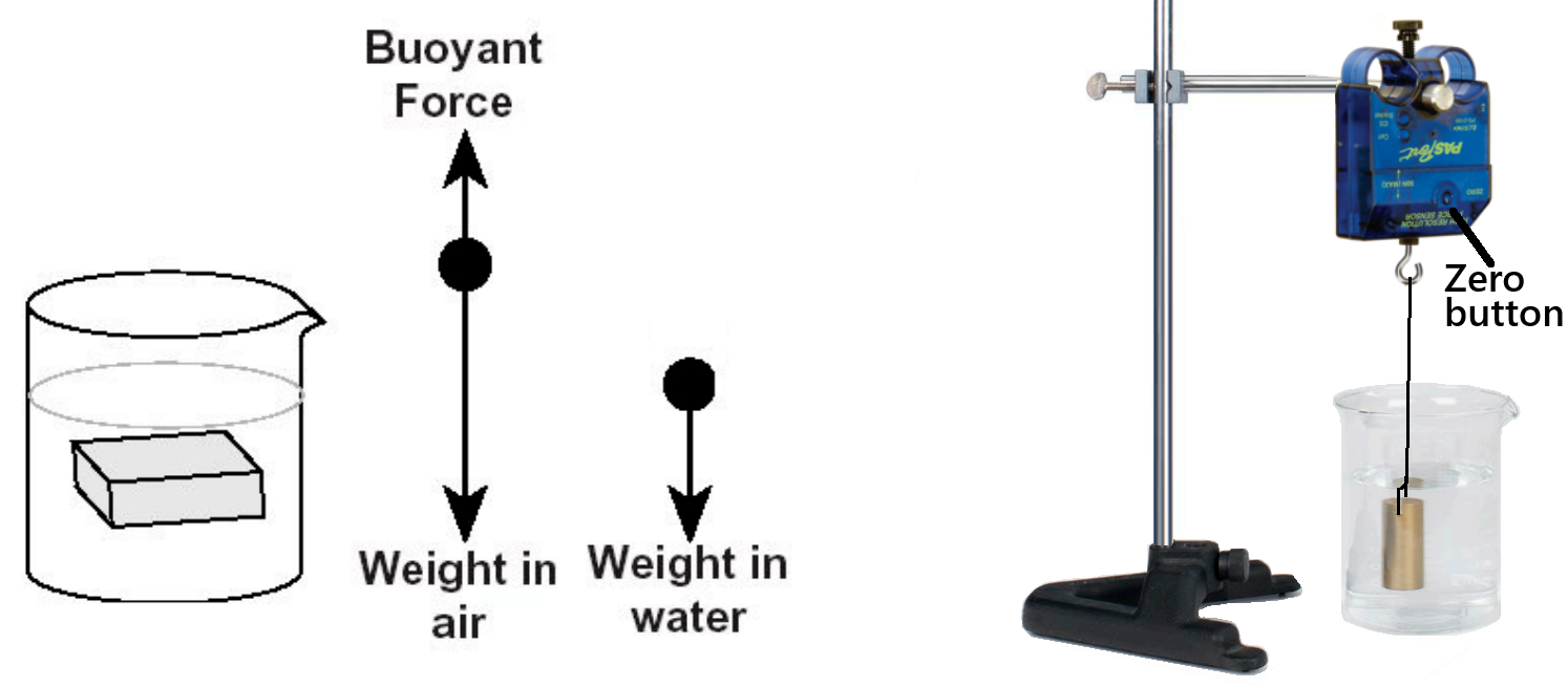
Figure 4:Left) Force diagram. Apparent weight in water is the difference of weight in air and buoyant force. Right) Force sensor measuring apparent weight of object in water.
When an object is submerged in a fluid, the apparent weight of the object is less than the weight in air because of the upward buoyant force (see Figure 4). Thus, the buoyant force can be calculated by finding the difference between the weight of the object in air and the apparent weight of the object when it is submerged in water.
○ Part I: Mass, Volume, and Density
Create a data table with:
Columns for the mass , volume , and density
Rows for each of the objects (clearly label or describe the objects in the table).
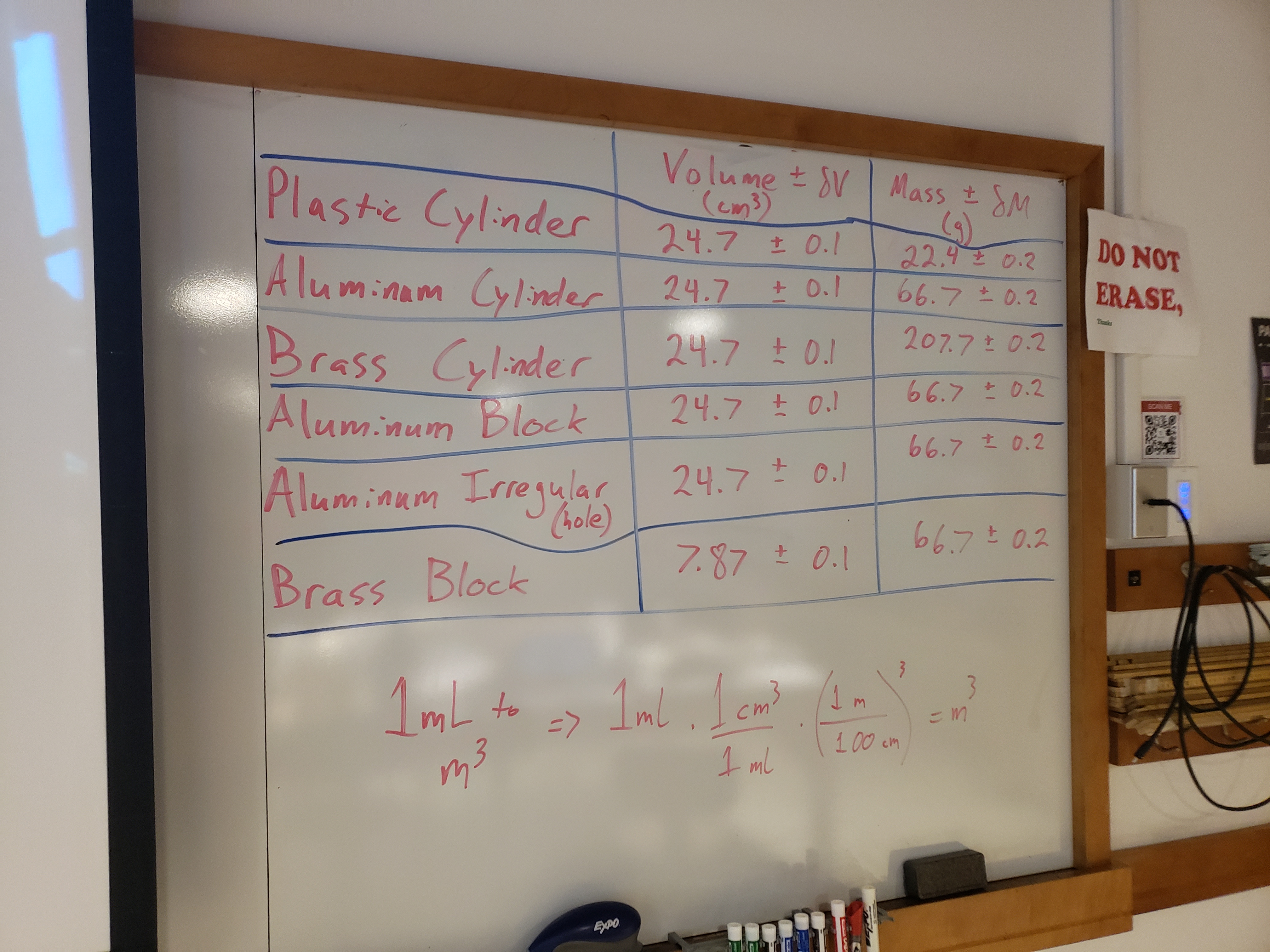
Record the mass and volume of each object into your spreadsheet. Normally, you would measure the volume and mass of each object (Figure 3) with Vernier calipers and a triple-beam balance, however, to save time during lab, the volume and mass of each object is presented here:
Table 1:Object Volume and Mass
Object Volume (cm) ± 0.1 Mass (g) ± 0.2 Aluminum Cylinder 24.7 66.7 Brass Cylinder 24.7 207.7 1/2 of Brass Cylinder 12.35 103.85 Brass Block 7.87 66.7 Aluminum Block 24.7 66.7 Aluminum Irregular (hole) 24.7 66.7 Plastic Cylinder 24.7 22.4
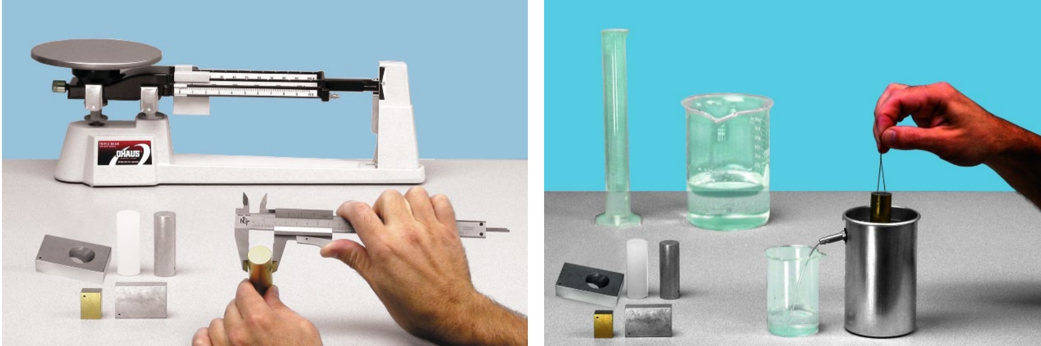
Figure 5:Left) Measuring size with calipers (not done in this lab). Right) Lowering object into overflow container.
In a separate area in your spreadsheet (like off to the right of your data table), list the objects in order from least to greatest mass.
In a separate area in your spreadsheet, list the objects in order from least to greatest volume.
In your data table, calculate the density of each object. In a separate area in your spreadsheet, list the objects in order from least to greatest density.
In a separate area in your spreadsheet, group the objects according to the type of material from which they are made.
○ Part II: Finding the Buoyant Force Using Archimedes’ Principle
For each of the objects, find the weight of the water displaced by each one:
Create a common data section and data table with:
Mass of beaker, for Fairfield, and other common data.
Columns including (but not limited to):
mass
weight
Rows for each of the objects plus the half-submerged brass cylinder. Clearly label or describe the objects in the table.
Find the mass of the beaker. After, place the beaker under the overflow container spout as shown in Figure 5.
Pour water into the overflow container until it overflows into the beaker. Allow the water to stop overflowing on its own and empty the beaker into the pitcher and return it to its position under the overflow container spout without jarring the overflow container.
If not already attached, tie a string onto each of the objects.
Lower the first object into the overflow container until it is completely submerged. Allow the water to stop overflowing. Measure the mass of the water plus beaker. Subtract the mass of the beaker to determine the mass of the displaced water. Multiply the mass by the acceleration due to gravity (9.803 m/s²) to find the weight of the water.
Repeat this procedure for the other objects. Note that the plastic cylinder will float so don’t try to completely submerge it in the water. Also find the weight of the displaced water when only half the brass cylinder is submerged.
List the objects in order from least buoyant force to greatest buoyant force.
○ Part III: Finding the Buoyant Force by Finding the Upward Force
Create a data table:
Seven rows for each of the 6 objects as well as the brass cylinder half-submerged (clearly label or describe the objects in the table).
Columns including (but not limited to):
: weight in air
: apparent weight in water
: buoyant force as determined with (9)
Ensure there is a loop of string attached to each object so they can be hooked onto the force sensor.
In Capstone, press record or monitor, and you will see the force in Newtons displayed (constantly updating). You can let this continue running to act as a continuous scale.
Before hanging any of the objects on the force sensor hook, zero the force sensor with the physical “zero” button on the front of the force sensor (shown in Figure 4).
With the water out of the way, record the weight of each object in air by hanging them on the hook.
Zero the sensor as needed if it appears to be drifting when swapping out the different objects.
Now place the pitcher of water beneath the force sensor such that when you hang each object from the force sensor hook, the objects can be fully submerged. Record the apparent weight of each object in water .
Calculate the buoyant force for each object by taking the difference between the weight in air and the weight in water with (9).
Add an additional column and calculate the difference (magnitude of difference in ) in between each method. (i.e. ).
Add an additional column and calculate for each object case the % difference between the buoyancy force (found here by measuring directly with the force sensor) and the buoyancy force found previously by Archimedes’ Principle of the displaced water.
● Bernoulli’s Principle (Second experiment)
○ Bernoulli --- Preliminary Setup
In our experiment, we will assume we don’t know the pressure at the constriction , and will use the Continuity and Bernoulli equations to determine experimentally what should be and compare to the actual value as measured by our pressure sensor.
The setup will be as in Figure 6. Water can be released from the pitcher sitting on the white/plexiglass box with the cooler-style spout as the release valve. On the other end of the water hose will be another release valve (at the bottom) for use during the determination of the flow-rate to rapidly stop the flow of water (if you only used the spout at the pitcher, much of the water would continue flowing out of the tube even after shutting if off, messing up the flow-rate calculations).
, as measured by the Quad Pressure Sensor, will be treated as a known actual or accepted value to be used in our calculations to solve for . It will be connected to port 1 (or port 3 if in the future these sensors break). We will calculate from our Continuity and Bernoulli Principle equations.
The value of , as measured by the Quad Pressure Sensor, will be treated as the known actual value to compare to. will be connected to port 2 (or port 4 if sensor is damaged).
After passing through the Venturi tube, the water will flow into a catch basin. There will also be a stopwatch to measure flow-rate during the first part of the experiment. If you require more water in your pitcher, use a separate pitcher to refill.
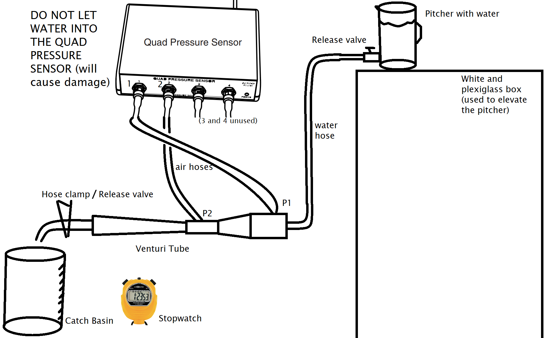
Figure 6:Sketch of the Venturi tube setup for the second experiment (Bernoulli).
○ Part I: Determining Flow Rate 
Create a data table:
6 rows for five trials of the measuring flow rate as well as the average flow rate and standard deviation of your flow rate .
Columns for the volume of water, elapsed time it took to flow, and flow rate .
With water in the pitcher, open the release valve (spout) to allow water to flow and remove all air bubbles within the tubing to achieve laminar flow. After a few seconds, close the bottom releave valve (after the venturi tube) at the end of the tube to halt the flow. Take whatever water is in the catch basin and return it to the pitcher.
Start current trial with the catch basin empty.
Start the stopwatch and open the bottom releave valve at the same time to start water flow.
After a measurable amount of water has flowed through, stop the stopwatch and close the bottom releave valve at the same time.
Measure the volume of water that flowed out of (or into) the apparatus (either with the scale on the catch basin or graduated cylinder).
Calculate the average flow rate for the current trial where is the volume of water and is the elapsed time.
Empty the catch basin or graduated cylinder back into the pitcher to keep a consistent amount of water in it.
Rerun this process starting with the empty catch basin (assuming the water hose is still clear of air bubbles) 4 more times for a total of 5 trials.
From the individual trial flow rates, calculate the average flow rate and standard deviation which we will use to represent our uncertainty in the flow rate ().
○ Part II: Determining Pressure at a Constriction (with Continuity and Bernoulli Equations)
Create a data table:
Common data section including:
Flow rate from Part I.
Cross-sectional areas and and their uncertainties and .
Velocities and .
Also include the maximum velocity at the wide () and minimum velocity at the narrow constriction () (Used to estimate pressure uncertainty later).
Density of water (use 998.2 kg/m for room temperature)
7 rows for:
five trials of the measuring and in Capstone as well as their averages and and standard deviations and .
Columns for and .
Determine the cross-sectional areas and of the wide and narrow constrictions respectively.
Reminder,
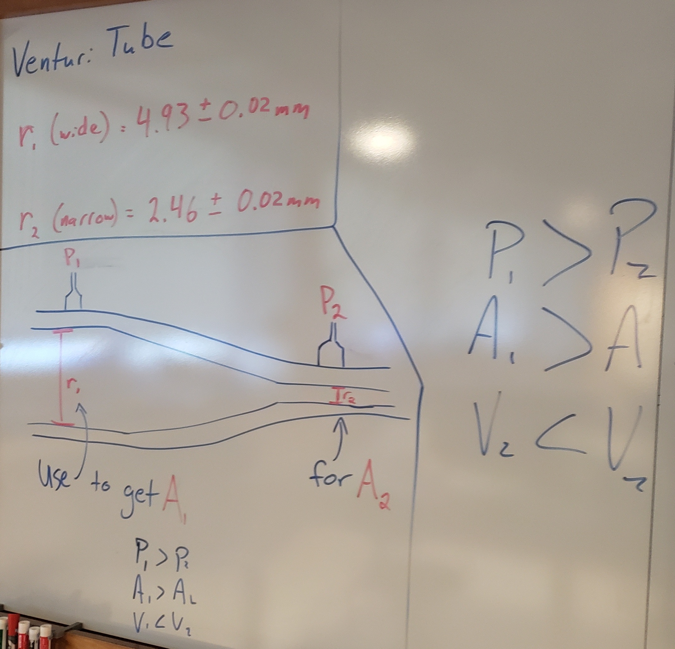
Radii values are provided to save time: at the wide, at the narrow (see The Whiteboard).
Determine the areas’ uncertainties and by maximizing the area using radii uncertainties (e.g. ) and taking the difference (e.g. ).
Calculate and with the Continuity (2) based on your determined areas and average flow rate.
Similarly, calculate MAXIMUM by maximizing the flow rate (e.g. ) and minimizing the areas (e.g. ).
Similarly, calculate MINIMUM by minimizing the flow rate (e.g. ) and maximizing the areas (e.g. ).
Capstone will be set up to show two pressures representing and . Double check that the pressure taps of the Venturi tube are appropriately connected like in Figure 6 where Channel 1 is connected to the wider part of the Venturi tube, and Channel 2 to the narrow constriction of the Venturi tube. (It’ll be easier to keep track of which pressure is which when the labels are similar.)
Capstone will also show a plot with both and on the y-axis as a function of time on the x-axis. To analyze either data set later on, you can click directly on the plotted data.
Calibrate the pressure sensor by:
Ensure both the top release valve and bottom releave valve are closed.
Disconnect the air hoses from the Quad Pressure Sensor via the quick connectors so the pressure sensors are open to atmospheric pressure. Set the air hoses to the side, ensuring at least part of the hoses are above the water level in the pitcher to prevent water from siphoning through the air hoses. The white bracket should provide this, but double check
In Capstone, select the green Calibration tab on the left-hand panel.
Pressure
Select all “Pressure Measurements”
Type of Calibration as “One Standard (1 point offset)”
Set Standard Value to average atmospheric pressure of 101.3 kPa --- Click the “Set Current Value to Standard Value” button
Finish
Both Absolute Pressure Channels 1 and 2, when you press record, should now read at about 101.3 kPa, if not, retry the calibration.
Ensure no water is near the end of the air hoses to prevent any water getting into the pressure sensors. Reconnect the air hoses to the pressure sensors. is marked with red tape.
You can open the hose clamp at the end of the hose as it will not be needed for the rest of this experiment. You will just need to catch basin to collect the water and avoid making a mess.
Press record, then open the release valve to allow the water to flow into the catch basin. After any air bubbles have passed and the water is flowing with minimal turbulence, continue recording pressure data for ~5 seconds, then close the release valve (spout) and stop recording.
Find the section of your Pressure vs. Time plot where flow was laminar (smooth without bubbles), should be a generally flat section of the Pressure vs Time plot. Click on the data on the plot, enable the highlight tool, and select a chunk of the plot when flow was laminar (no bubbles, the flat part). Do the same for the data. You can find the average value for and at the bottom of the table on the left hand side of your screen, where the mean is representing the average value of whichever subset of the data you’ve highlighted.
Record both and . There should be a difference of ~2--5 kPa, if not, double check that the pressure tubing was properly reconnected and water is flowing was flowing. As needed, check with an instructor.
Rerun this process from Step 21 an additional 4 times for a total of 5 trials.
Determine the averages and values from your five trials. Also determine their standard deviations and .
Calculate your experimental value of with (6) using your previously determined velocities and and your average treated as the known actual value for the wider part of the Venturi tube.
Similarly, for estimating an uncertainty in your average experimental value in the next step, calculate your max experimental value of by maximizing (e.g. ) and using your already determined maximized or minimized velocities and .
Represent your uncertainty with the difference of your maximized value and average values:
BEFORE CLOSING CAPSTONE:
BEFORE LEAVING LAB:
Post-Lab Submission --- Interpretation of Results
● Finalized Spreadsheets
Make sure to submit your finalized data table (Excel sheet).
Please include for discussion relevant screenshots of your Capstone plots including:
1 plot of and vs. Time (just 1 trial) --- note where you are measuring.
● Archimedes’ Principle --- Post-Lab Error & Results Analysis
In a paragraph, summarize your error analysis. Be both qualitative and quantitative.
Where might errors arise in measuring the buoyant force?
What are your measurement uncertainties for each experiment?
What are possible systematic uncertainties for each experiment?
How do these uncertainties affect your final results for ?
In a paragraph, summarize the results you have determined in each case. Consider:
In which list (mass, volume, or density) are the objects grouped similarly?
In each object case, compare the the buoyant force determined from each method --- Part II was with displaced water for , Part III was direct force sensor measurements for . Were they equal? How different were they?
Were the % differences between the two methods for each case relatively small, consistent, or did any case standout?
Which objects had the same buoyant force when submerged? Why?
For the plastic cylinder, what was the apparent weight in water? What would be the buoyant force be if plastic cylinder were completely submerged?
How did the buoyant force for the totally submerged brass cylinder relate to the buoyant force for the half-submerged brass cylinder?
What does the buoyant force depend on: The mass of the object, or its volume, or its density, or the material from which it is made?
● Bernoulli’s Principle --- Post-Lab Error & Results Analysis
In a paragraph, summarize your error analysis. Be both qualitative and quantitative.
Where might errors arise in measuring the flow rate?
What are your measurement uncertainties for each experiment?
What are possible systematic uncertainties for each experiment?
What errors might cause your to diverge from ?
In a paragraph, summarize the results you have determined in each case. Consider:
Does your experimental value for agree with the actual value of as measured with the pressure sensor? (i.e. does overlap with ?)
How is the Bernoulli Principle different than the Bernoulli Equation?
What assumptions about the fluid allows the Bernoulli Principle to work? (i.e. what type or characteristics of the fluid and/or flow are necessary assumptions for Bernoulli to hold true?)
Imagine that instead of being on the table, the Venturi tube were set on the floor with the rest of the experimental apparatus unchanged. Would the difference in pressures we see on the Capstone plot between and during the smooth, laminar flow section that we analyzed to find average pressures be larger, smaller, or the same. Why?
The Whiteboard