Centripetal Force with Mass on Rotating Arm
Background
● Background Overview
Acceleration is the rate of change of velocity. An object moving in a circle of radius is always being accelerated even if its speed remains constant. This is because velocity is a vector quantity whose direction is continuously changing. This rotational change in direction requires a centripetal force that is pointed in towards the axis of rotation (center-seeking). The corresponding centripetal acceleration also points toward the axis of rotation with a magnitude . For an object of mass , the required force for this circular motion is thus related quadratically to the speed of the object and inversely to its radius of curvature:
For each case, the object’s mass and radius are set by attaching small masses to a freely-sliding holder on the rotating arm (shown in Figure 1). The tangential speed of the object is obtained from the rate at which a small white-ish pin beneath the fixed-in-place counterweight holder passes through the photogate. The centripetal force is determined by measuring the force in the cable with a force sensor (seen later in Figure 2). Subsequently, the is determined from graphs relating vs. and vs. . The procedure is repeated for different masses and radii to study how centripetal force depends on velocity.
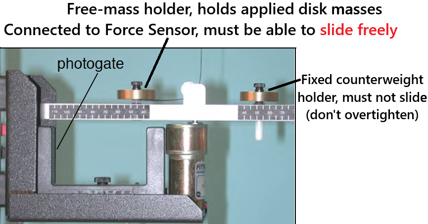
Figure 1:Experimental Setup showing the rotating arm and the attached masses. The photogate to measure the speed is shown as well. The small white-ish pin attached underneath the fixed-counterweight mass holder is used to determine the speed of the mass.
Experimental Procedure
● Procedure Preview
● Preliminary Setup
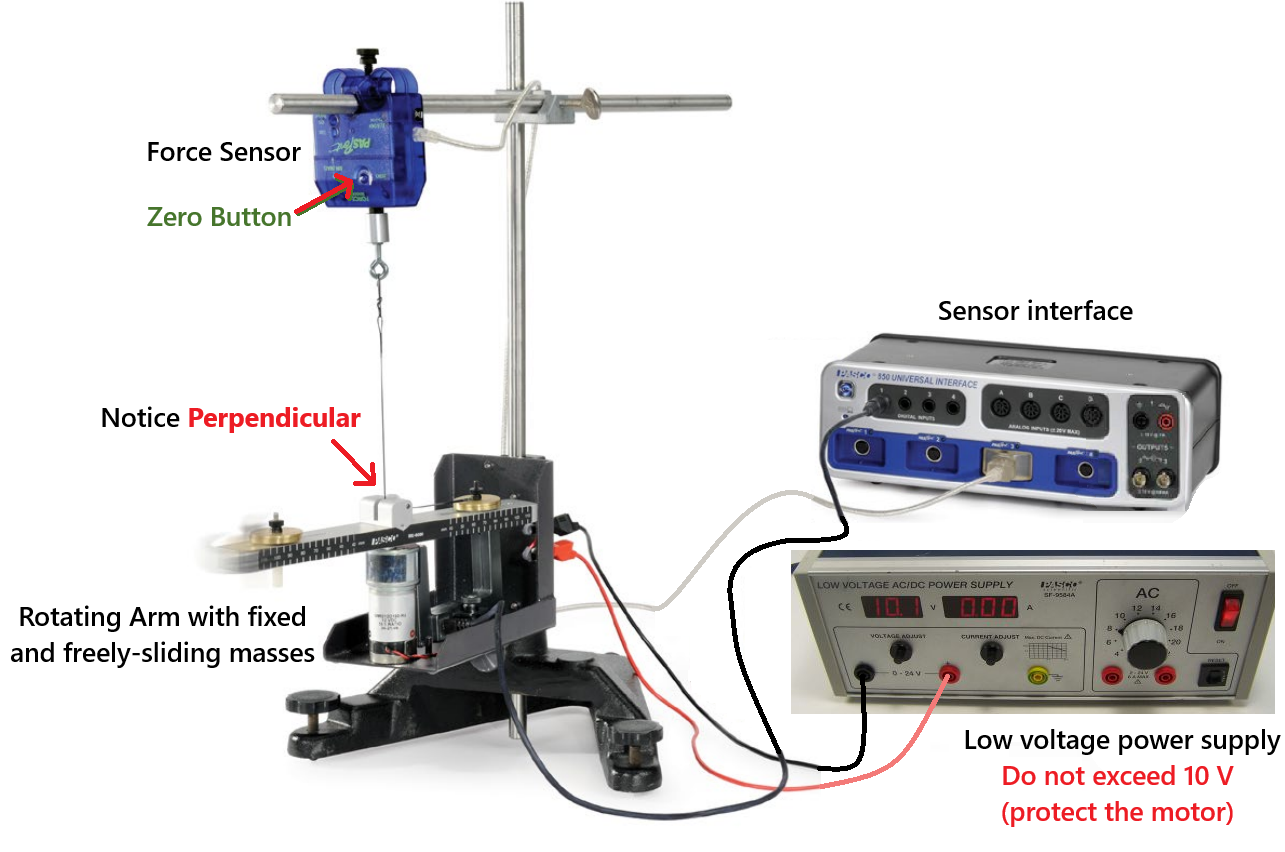
Figure 2:Experimental Setup for the centripetal force experiment
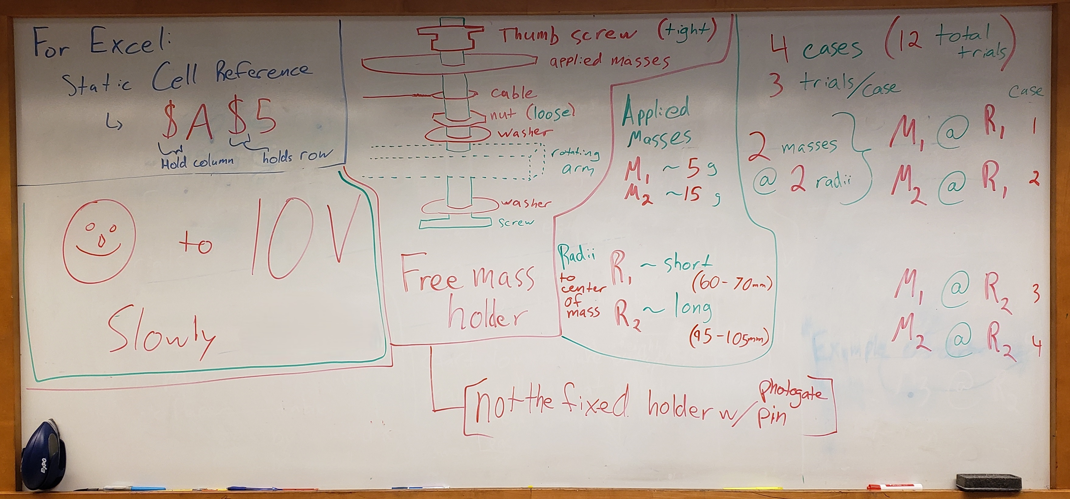
The experiment should already be setup for you as shown in Figure 2 with masses attached to both the freely-sliding and fixed-counterweight mass holders as well as already being hooked up to the computer interface and power supply. Reminder, the relevant Capstone file will be on the desktop (e.g. Figure 3). Prepared are relevant notes, a stopwatch, and two graphs:
versus
versus
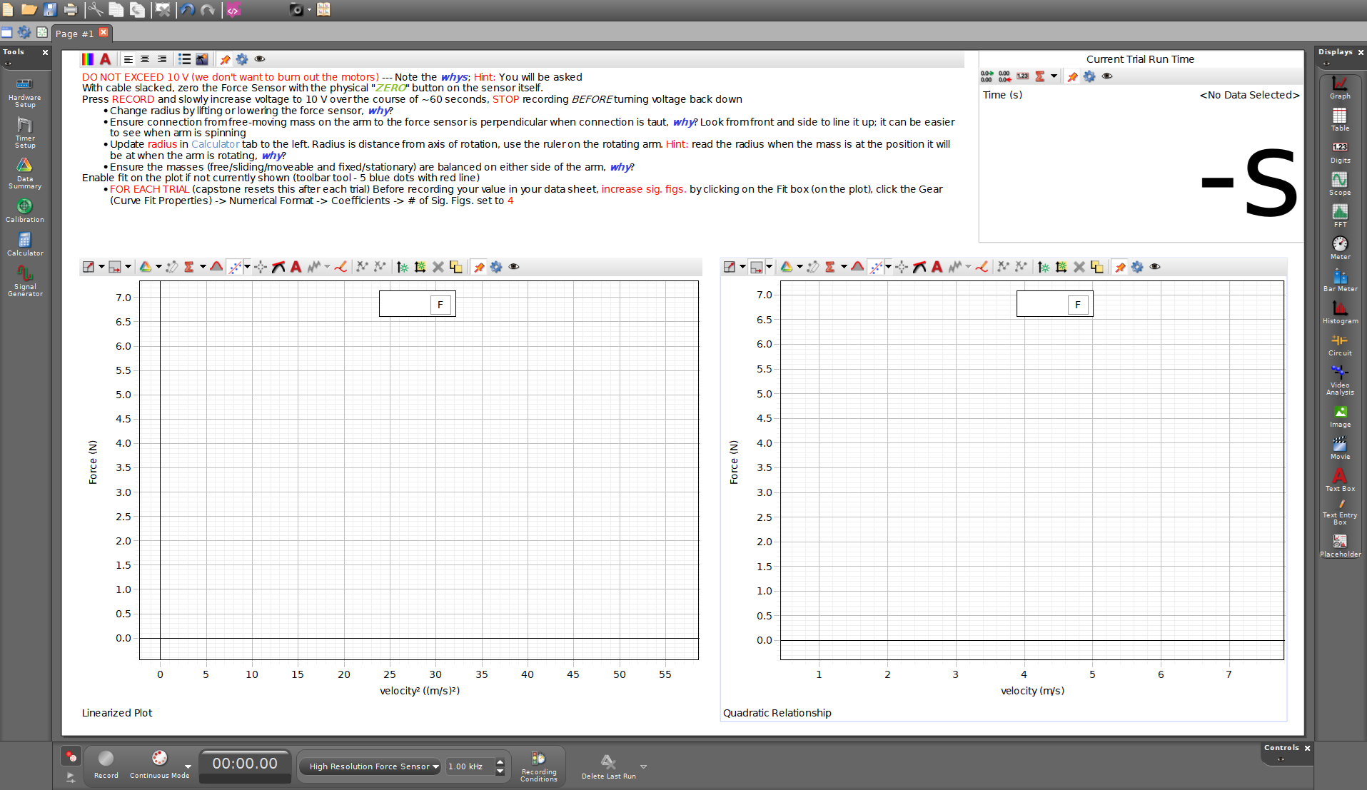
Figure 3:Example of today’s Capstone layout. Review notes for helpful info.
Create a overall common data table including (but not limited to):
the mass of the freely-sliding mass holder (kg)
uncertainty of the mass of the freely-sliding mass holder (kg)
Remove the freely-sliding mass holder and measure its mass with a triple-beam balance. Record this in your data sheet. Re-attach the assembly to the rotating arm with one plastic washer below the arm and one above. Then the silver nut, tightened down enough to prevent tipping, but the assembly must slide freely. Then the cable loop. Then use the black nut to attach the applied disk masses above the loop. See order in Figure 4.
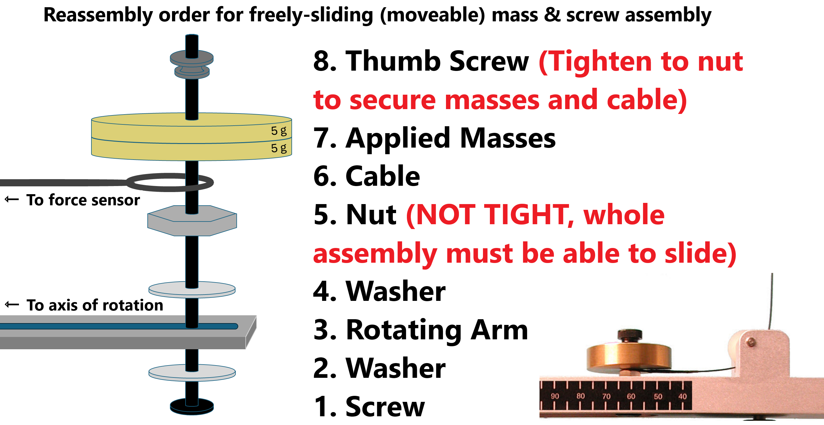
Figure 4:Reassemly procedure for reattaching the freely-sliding mass holder
Four cases will be performed, each with 3 trials, as listed in Table 1. For each of the four cases, perform the following steps listed in ● Experimental Data Collection and record the data appropriately in your spreadsheet.
Table 1:Four experimental cases applied masses and radii
Case Applied Mass (g) Radius (mm) 1 5 LONG () 2 15 LONG () 3 5 short () 4 15 short ()
● Experimental Data Collection
For each case, construct:
A common data table for the current case including (but not limited to):
: mass of applied disk masses (kg)
: actual mass of the rotating, freely-sliding object
: the radius (m)
: your estimate of the uncertainty in the radius (m) (i.e. )
A data table with a row for each trial, average values, error-maximized “trial” for error propagation later on as well as columns for (but not limited to):
: fit parameter from the vs. (linear fit)
: the mass determined from vs.
the difference between and
: fit parameter from the vs. (quadratic fit)
: the mass determined from vs.
the difference between and
Additional section for:
the uncertainty in the mass from the centripetal force due to your estimated radius uncertainty (Point to consider: how much does the derived mass change if you change your value for radius in Capstone calculator by the amount of your estimated radius uncertainty?)
Attach the necessary applied masses for the current case as listed in Table 1 following steps depicted in Figure 4. Record . Calculate the total mass of the rotating object (i.e. the sum total of the freely-sliding mass holder and the applied mass).
Set radius to the value listed in Table 1 for the current case; it just needs to be within the range listed. Do this by raising or lowering the force sensor (see bar & clamp holding force sensor in Figure 2). It is important that the force sensor be exactly above the center of the apparatus. To check this, pull on the freely-sliding mass to put tension in the cable. Then observe the cable from the front and side of the system to verify it is parallel to the L-stand’s vertical rod and perpendicular to the rotating arm. Adjust the horizontal rod holding the force sensor until that is that is achieved. Ensure the force sensor is still pointed downwards towards the pulley at the axis of rotation. Any time you change the position of the Force Sensor, you will have to repeat this step.
Measure and record radius . Pull the mass to tighten the cable to determine the actual radius to the nearest millimeter. You can do this using the scale attached to the side of the apparatus.
Estimate , your estimated uncertainty in the radius. Remember, this is a bit subjective relating to how confident you are that the freely-sliding object is at your stated radius, not soley the precision of your tools. It essentially becomes how far you could move the object a bit towards or away from the axis of rotation, and still be confident in saying your radius measurement is accurate. Also consider how stiff the attachment cable is; does that impact how constant the radius is during rotation?
Set the radius in Capstone’s Calculator which is set up to determine instantaneous tangential velocity. Select Calculator in the menu on the left-hand side (example shown in Figure 5). In line 1, replace the
0.###value with the value that you actually measured in the previous step. Click the Calculator again to close it. Any time you change the radius, you will need to update the value in Calculator.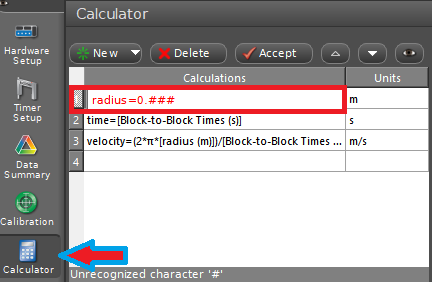
Figure 5:Calculator setup in Capstone to determine the tangential speed of the rotating objects. Adjust the radius (red boxed) to your measured radius in your experimental setup.
To avoid wobbling, tighten an identical fixed-counterwieght mass to the opposite side of the rotating arm such that it is as far from the axis of rotation as your previously measured . Tighten so it doesn’t move --- DON’T OVERTIGHTEN, THIS CAN DAMAGE THE RUBBER WASHERS.
ZERO the force sensor:
Press Record. Wiggle the rotating arm such that the white pin underneath the counterweight passes back and forth through the photogate. It is likely the force sensor is not calibrated yet, and you might see values for the force on the left-hand linear graph not plot on the .
ZERO the force sensor with the physical ZERO button on the force sensor while ensuring the connecting cable is slack.
You can check the force sensor is now zeroed out by again wiggling the rotating arm to cross the photogate and find that the data points are now plotting on the . If this is not the case, try again until it does.
You can stop recording and ignore that data.
Double check the force sensor calibration as needed, including after changing the radius.
Start the data acquisition in Capstone by pressing the Record button. You should notice that the program might not show values; this is normal as it will only record a value once the photogate has been crossed by the white pin underneath the fixed-counterweight.
Over the course of about 60 seconds (see stopwatch in top right of Capstone, e.g. Figure 3), slowly increase the voltage on the power supply from to . The metal arm will begin to rotate, and you will notice the graphs display the data as it is collected. You may notice kinks in the data (e.g. Figure 6); that is alright as some power supplies may have small jumps in the voltage as it switches to different internal circuits. If there is a kink, what does that represent? For your trial, focus on slowly and consistenty increasing the voltage.
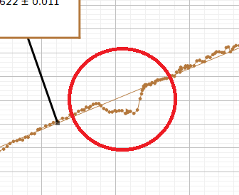
Figure 6:Example of kink in the data due to possible irregularities or voltage jumps in the power supplies.
Before returning the power supply to zero, press the STOP button in Capstone to stop data acquisition. When you are finished taking data, you can scale both axes of either graph using the tool shown in Figure 7.

Figure 7:Autoscale axes tool.
Once you have finished your trial:
Fit a straight line to your vs. graph and set its y-intecept to zero. Note: you will need to do this for each trial as Capstone resets to the default settings for each trial. For visual instructions, see Figure 8. Select the fit box select Curve Fit Editor lock the y-intercept update the fit. Notice the change in slope when you lock .
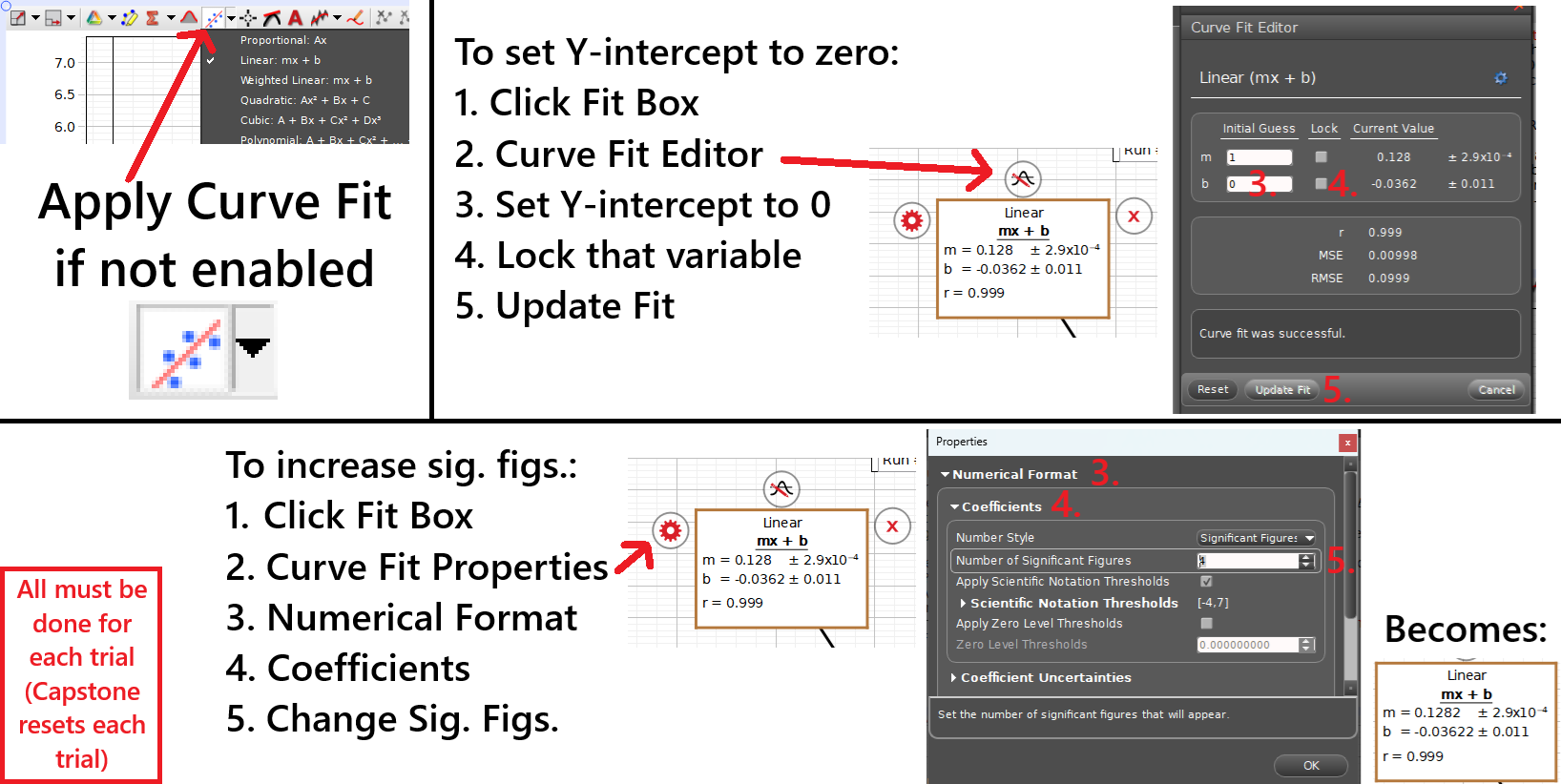
Figure 8:Process for applying fits to plotted data, updating the y-intercept and other curve-fit terms, and updating sig. figs.
Increase the number of significant figures in for the fit. Note: you will need to do this for each trial. For visual instructions, see Figure 8. Select the fit box select Curve Fit Properties (gear) Numerical Format Coefficients update sig. figs. to at least 4.
Record , the linear fit’s slope in your data table (based on ).
Calculate your experimental mass of the rotating object based on your linear fit using (1).
Calculate the difference between your experimental and the actual mass .
Fit a quadratic curve to your vs. graph and set its coefficients and to zero y-intecept to zero in a similar fashion to your linear plot. Note: you will need to do this for each trial. For visual instructions, see Figure 8. Notice the change in coefficient when you lock and .
Increase the number of significant figures for the quadratic fit to at least 4 in a similar fashion to the linear plot. Note: you will need to do this for each trial. For visual instructions, see Figure 8.
Record , the first term’s coefficient in your data table (based on ).
Calculate your experimental mass of the rotating object based on your quadratic fit , again using (1).
Calculate the difference between your experimental and the actual mass .
Repeat the previous steps of ● Experimental Data Collection for rest of the trials for this current case, then continue to the analysis of the current case in the next sections: ○ Combined Results for Current Case and ○ Error Propagation for Current Case.
○ Combined Results for Current Case
Calculate the averages of all your previously determined values in your data table for the current case.
By now, we should see that when we force both linear and quadratic fits to the origin, . If not, please discuss with your instructor.
Assuming they are equal, the average mass of the rotating object will be written as (the bar over the represents the average value). In the next section, ○ Error Propagation for Current Case, you will propagate measurement uncertainty(ies) to determine the uncertainty in your average experimental mass
○ Error Propagation for Current Case
Over the next few steps, use error propagation to determine uncertainty in your average mass of the rotating object :
A. Using just 1 of your trials from this case, determine the propagated uncertainty in the experimental mass of the rotating object by maximizing the by . See how that changes the graph, determine the maximized or minimized error-test mass , take the difference between the error-test and trial mass values, and treat that difference as for this case (rather than doing all trials to save time).
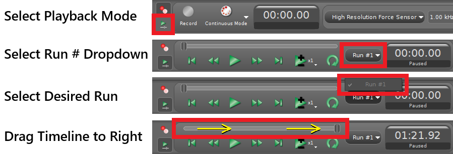
Figure 9:Process for returning to previous run in Capstone.
B. Essentially create an additional trial for this case in a new row in your data table.
C. Return to the calculator (Figure 5) and update the radius to be larger or smaller based on your values . Notice how your graphs and fits change.
D. Use those updated values in this error-test trial to determine . Notice how the experimental mass of the object changes (maximized or minimized). Reminder: you updated the radius in Capstone; how did you then determine mass?
E. Determine the uncertainty in your selected trial’s experimental mass as the magnitude or absolute value of the difference between the error-test and trial values for object’s mass:
F. Treat this difference as your uncertainty in your average mass of the rotating object, .
Repeat the previous steps in ● Experimental Data Collection for the next case with the relevant applied mass and radius as listed in Table 1. Please call for help as needed for setting up next cases.
BEFORE CLOSING CAPSTONE:
BEFORE LEAVING LAB:
Post-Lab Submission --- Interpretation of Results
● Finalized Spreadsheets
Make sure to submit your finalized data table (Excel sheet).
Please include relevant plot(s) including:
A screenshot or photo of the linearized and quadratic plots from Capstone for just one trial for discussion purposes.
● Post-lab Writeup
In a paragraph, summarize your error analysis. Be both qualitative and quantitative.
What is the precision of your equipment?
What are possible random errors for today’s experiment?
What are possible systematic errors for today’s experiments?
Discuss your uncertainties (see ○ Error Propagation for Current Case) and their effects
Sources of measured or estimated uncertainties (values); how large are they?
How do they affect your final mass values; what has the largest affect?
In a paragraph, summarize the results you have determined in each case.
From where did you determine your experimental mass? Do your experimentally determined masses with uncertainties () agree with the actual mass of the applied masses plus mass holder (i.e. range overalapping with actual value)?
How does the shape of the vs. plot compare to the vs. plot?
What does this tell you about the mathematical relationship between centripetal force and velocity?
For example, if the velocity is doubled, does the centripetal force also double, or does it change by a different factor? What is that change in centripetal force?
Why should there be the same mass on the fixed-counterweight mass holder as compared to the freely-sliding mass holder? What might you expect to see in your data if the fixed-counterweight and freely-sliding masses and radii were not comparable?
The Whiteboard