Resistivity with Resistors & DC Circuits
Background
● Background Overview & Resistance
If a potential difference is applied across some element in an electrical circuit, the current in the element is determined by a quantity known as the resistance . The relationship between these three quantities serves as a definition of the quantity resistance :
An object that is a pure resistor has its total electrical characteristics determined by (1). Other circuit elements may have other important electrical characteristics in addition to resistance, such as capacitance or inductance. The resistance of any circuit element, whether it has other significant electrical properties or not, is given by the ratio of voltage to current as described in (1). For any given circuit element, the value of this ratio may change as the voltage and current changes. Nevertheless, the ratio of to defines the resistance of the circuit element at that particular voltage and current. The unit of resistance is the volt/ampere defined as the ohm, denoted by the symbol “.”
● Ohm’s Law
Certain circuit elements obey a relation that is known as Ohm’s Law. For these elements, the ratio of to (i.e. ) is a constant for different values of . Therefore, in order to show that a circuit element obeys Ohm’s Law, it is necessary to vary the voltage (the current will then also vary) and observe that the ratio is in fact constant. In today’s experiment, such measurements will be performed on two different types of elements to determine their resistance response to voltage (ceramic/metal-film resistors and an incandescent light bulb).
● Resistivity & Temperature Dependence
The resistance of any object to electrical current is a function of the material from which it is constructed, as well as the length, cross-sectional area, and temperature of the object. At constant temperature, the resistance of a sample with a constant cross-section , and length is given by
where is a material constant called the resistivity. Normally is dependent upon the temperature of the sample; depending upon the material, may either increase or decrease with increasing temperature. Thus, if the current is sufficient, the heating of the material by the current passing through it can change the resistance.
Consider a “black box” with some unknown circuit inside connected to two terminals on the box. If we apply a voltage to the terminals and observe a current flowing through the “black box,” we define the resistance of the “black box” to be . If the resistance of the circuit element is a constant independent of both the current and the voltage, then we say that the circuit element is ohmic and that it follows Ohm’s law. Georg Simon Ohm found that most pure metals at room temperature have this property. However, a light bulb has a tungsten filament that heats up as you increase the current through it. Since the resistance of tungsten increases with temperature, the resistance of the tungsten filament increases as the voltage increases. Therefore a light bulb does not follow Ohm’s law.
For an ohmic resistor, when a voltage is applied, then the current is , so the current is proportional to the voltage. If you plot voltage vs. current, the result is a straight line whose slope is the resistance. For a non-ohmic element like a light bulb, a plot of voltage vs. current is curved.
● Series & Parallel Circuits
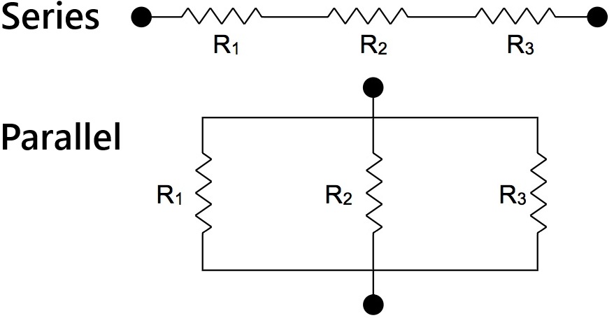
Figure 1:Resistors connected in Top) Series, one after the other/end to end, making a LOOP, Bottom) Parallel, all connected to the same starting and ending JUNCTIONS.
Series and parallel connections for three resistors (, , ) are illustrated in Figure 1.
The equivalent resistance for each of these networks is that resistance which can replace the network of resistors between the terminals of the network. for each is given by:
○ Series Circuits --- Kirchhoff’s Voltage Rule
Notice, in a series circuit, if voltage is applied, the current flows the same through every element. The sum of the voltage drops across the elements equals the applied voltage. This follows from conservation of energy and is expressed by Kirchhoff’s Voltage Rule (a.k.a. Loop Rule):
The algebraic sum of the voltage changes around any closed loop is zero.
In this experiment, you will primarily verify that the measured voltage drops across series elements add up to the total applied voltage, and secondarily confirm current is consistent through each element.
○ Parallel Circuits --- Kirchhoff’s Current Rule
In a parallel circuit, if a voltage is applied, the voltage across each branch of the circuit is the same. The total current flowing into or out of a junction equals the sum of the currents through each branch. This follows from conservation of charge and is expressed by Kirchhoff’s Current Rule (a.k.a. Junction Rule):
The sum of currents into a junction equals the sum of currents out of the junction.
In this experiment, you will primarily verify that the measured branch currents add to the total circuit current, and secondarily confirm voltage drops across each element is consistent.
Kirchhoff’s Rules above provide the equations needed to determine unknown currents and voltages in complex circuits. In this lab, you will apply these rules to analyze series and parallel resistor networks.
● Equipment
Overall setup shown in Figure 2, with a full equipment list in the following table Table 1.
Table 1:Equipment
| Category | Items |
|---|---|
| Power Supply | • PASCO 850 Universal Interface (~0–6 V DC) • Capstone example Figure 6 |
| Resistors | • 3x ceramic/metal-film resistors (< 1 ; blue, gray, brown) (Figure 3) • 1x light bulb — DO NOT EXCEED 6 V (Figure 3) |
| Connections | • 9x jumper bars (Figure 3) |
| PASCO Modular Circuit Kit | • 1x light bulb module • 12x spring clip modules (attach resistors, voltmeter, ammeter; build series/parallel circuits) • 1x SPST switch module (open/close circuit) • 1x red/black terminal module (connect to DC supply) • 11x T-junction modules • 5x straight-line modules • 4x blank modules • 34x U-shaped jumper clips |
| Measurement Device | • Fluke multimeter with alligator clips (Figure 5) • : measure resistor & bulb resistance (Figure 4 left) • DC V: measure voltage drop across circuit elements (Figure 4 center) • DC A: measure current through resistors & bulb and series & parallel circuits (Figure 4 right) |
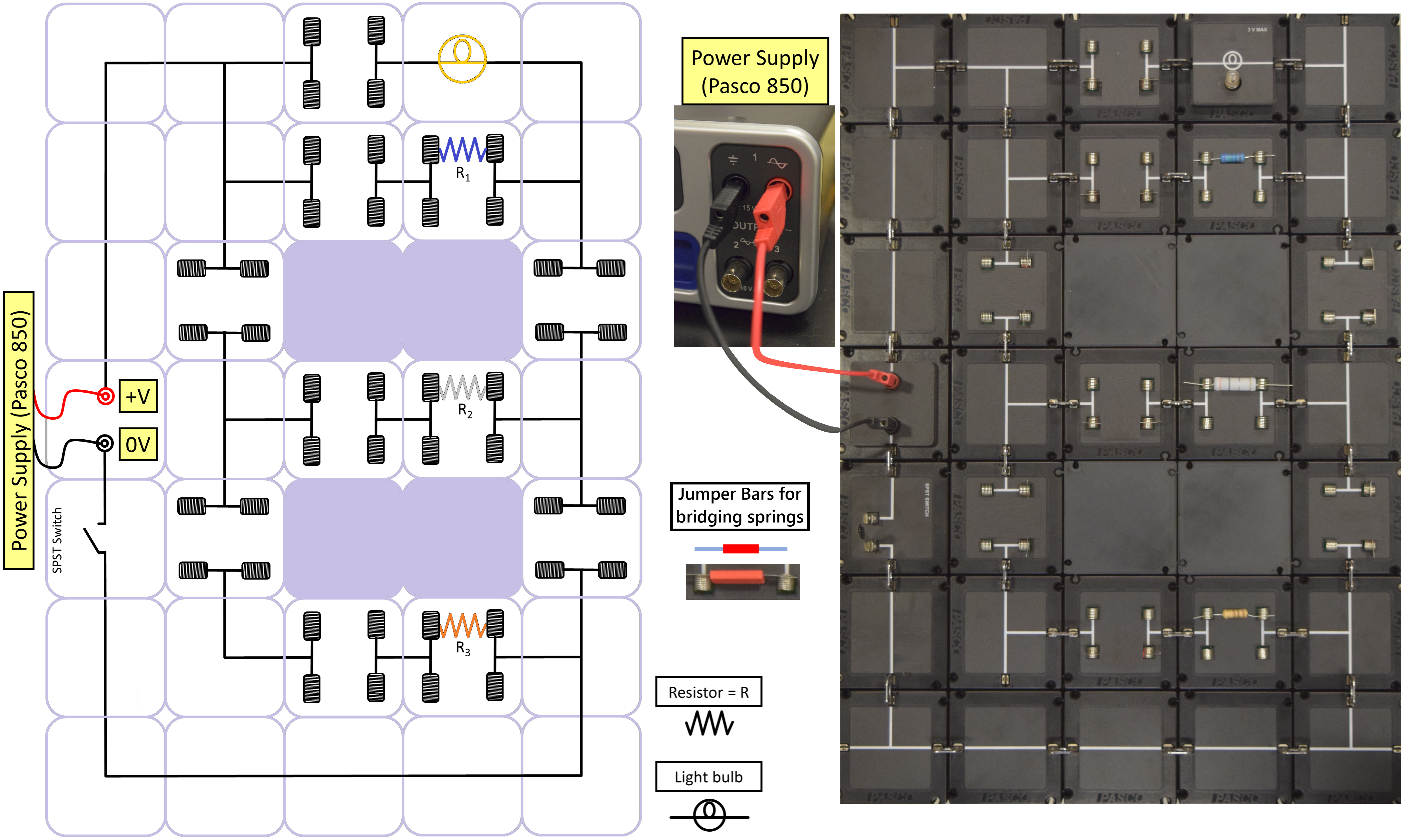
Figure 2:Left) Schematic, with circuit modules with light bulb and the three resistor locations noted. Right) Example of actual setup with resistors installed (they can stay in these positions for the whole lab and do not need to be moved around). Red jumper bars can be added or removed to create different circuit configurations. Light bulb and resistor locations are shown for easy testing. Power is supplied by the black and red banana plug output from the Pasco 850 (controlled in Capstone). SPST switch can be used to open/close entire system.
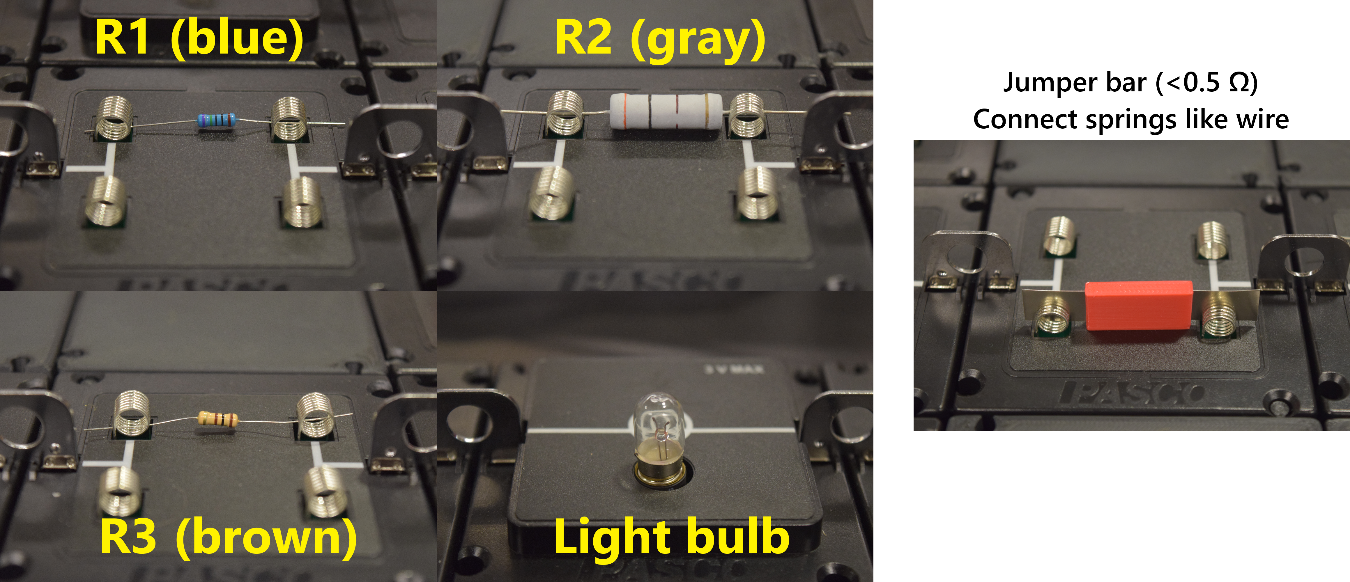
Figure 3:Examples of the resistors, light bulb, and jumper bar you will use today. They can stay in their same spring modules for all parts of the lab today.
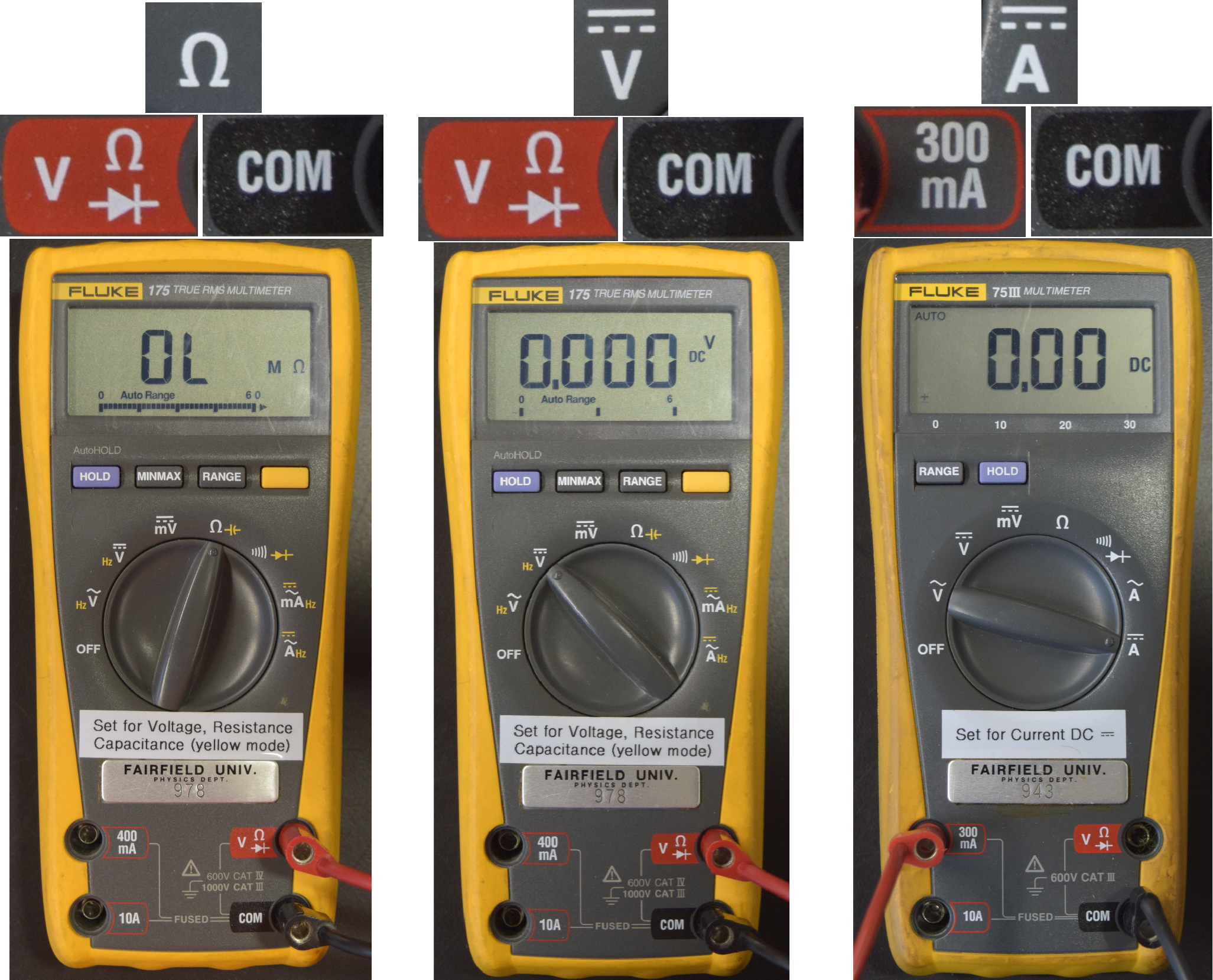
Figure 4:Examples of the measurement type, connections used, and multimeter overall configurations in use today. There are 2 Multimeters in use, one for BOTH Resistance and Voltage, one for JUST Current. Left) configuration for measuring resistance in ohms --- note, this auto-ranges, double check the magnitude of your units (e.g. , , ). Center) configuration for measuring DC voltage in volts (V). Right) configuration for measuring DC current in milliamps (mA) through the 300 mA fused circuit.
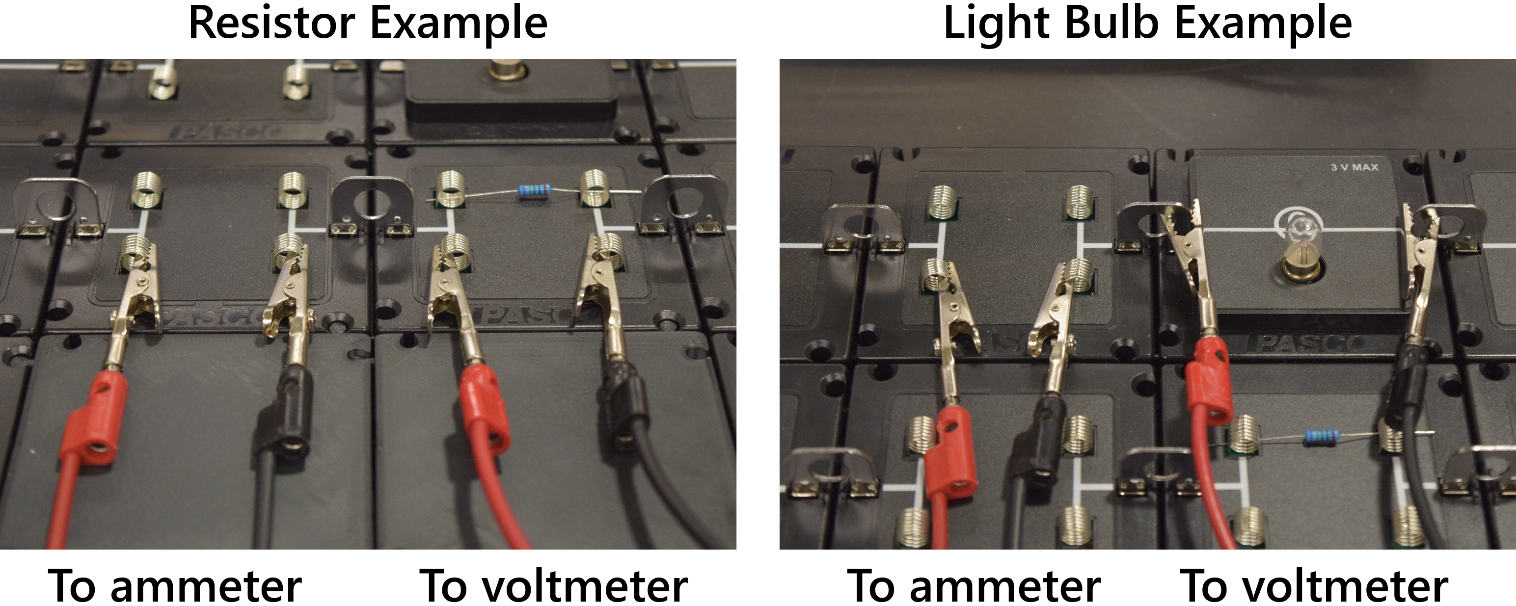
Figure 5:Examples how to connect ammeter (in line or in series with resistor) and voltmeter/ohmmeter (across or in parallel with resistor) alligator clips to the spring modules. For the light bulb, connect voltmeter to the U-shaped module clips.
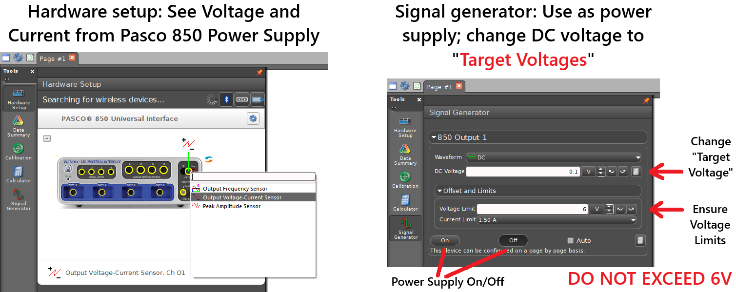
Figure 6:Example of Hardware Setup, selecting Output Voltage-Current Sensor, and Signal Generator tabs in Capstone set to DC waveform, control output voltage with “DC Voltage”, Voltage limit of , Current limit of , use On/Off buttons to supply power. Not Shown) Voltage and Current Monitored output --- purely just for making sure Capstone is providing power and working, not for any measurements (those will be made with the yellow multimeters).
Experimental Procedure
● Procedure Preview
● Preliminary Setup
Create a common data table of your resistors’ resistances in Ohms () where , , , and .
Measure and record to the common data table the actual resistances of each ceramic/metal-film resistor and light bulb as , , , .
Take such measurements with the Fluke ohmmeter (setting as shown in Figure 4 left, will be the same multimeter you use later for just voltage). You will compare your experimentally determined values to these later on.
To measure their resistance, you can either attach the alligator clips directly to the ends of the resistors and light bulb, OR more preferrably to decrease wear and tear, place the resistors in the spring modules as you will in the next step, and connect the alligator clips to the springs or U-shaped clips as shown for the voltmeter connections in Figure 5. This second method is preferred as it is generally easier to deal with, especially for the light bulb.
Also record an uncertainty in your actual values for each resistor and light bulb in the common data table. (hint: how are you measuring, where would the uncertainty come from for this measurement?)
Prepare your experimental set up to match the example Figure 2, with light bulb, , , and in their respective positions. Attach the resistors by gently sliding the wire leads into the springs of the spring modules as shown in Figure 3. Connect the banana-plug wires if not already connected from the DC power output as supplied by the Pasco 850 interface to the red/black terminal module. Red-handled jumper bars are to be treated like wires that bridge the air gap of the springs and continue the electrical connections.
● Part I -- Individual Resistors across Voltage Range
For the first resistor, , build your closed-loop ciruit with just plus jumper bars and ammeter (WHICH ELECTRICALLY ACTS LIKE A JUMPER BAR BY ALLOWING CURRENT TO FLOW THROUGH IT TO MEASURE CURRENT FLOW). Add/remoce jumper bars as needed to bridge the air-gapped spring modules (if a jumper bar is installed, current will take the jumper bar path). It will be the same as what is shown in the schematic of Figure 7. TRACE WITH YOUR FINGER the circuit from start (red terminal) to finish (black termial) to ensure the circuit is closed for . Starting from the red (positive) terminal to of the red/black terminal module, make sure your circuit goes through to the ammeter, across the resistor, across any needed jumper bars, ensure SPST switch is closed, and end back at the black (negative) terminal. If you find a gap that you need to cross, add jumper bars as needed. Ensure ammeter and voltmeter are connected to measure current through and voltage drop across the resistor (see Figure 5). (Note: no jumper bar needed for ammeter connections as we want the current to flow through the ammeter, not bypass it on the jumper bar)
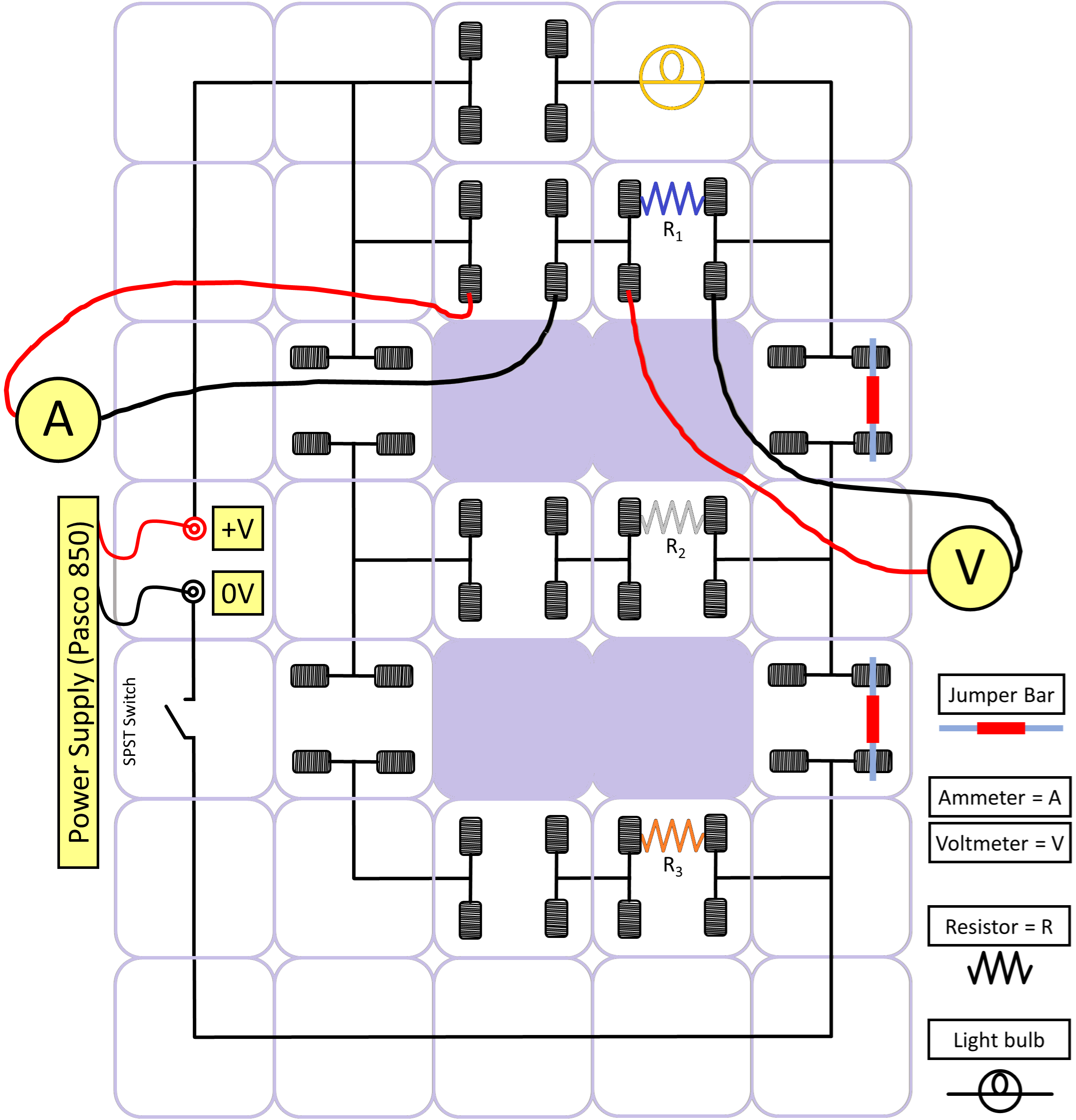
Figure 7:Schematic example of a circuit for with jumper bars in place to make the necessary electrical connections across the spring modules to make a closed loop from power terminal (red) to power terminal (black). See how the ammeter acts like a jumper bar connecting springs and allowing current to flow through it. See how the voltmeter connects to either side of the resistor and measures how much the resistor causes voltage to drop.
For the first resistor case, create a data table with columns for the following list (but not limited to; add columns as needed for unit conversion to SI units) and include enough rows for each trial/target voltage:
Trial number
Target voltage: increments you set in the Capstone power supply
Measured voltage: voltage drop across circuit element in question
Measured voltage uncertainty
Measured current: current flowing through circuit element in question
Measured current uncertainty
Resistance: resistance as calculated with Ohm’s law
Additional areas for
LINEST()calculations later on.
Target voltages will be . The first trial is the odd one out since we want a near-zero value, but cannot actually be at zero volts.
On the lab computers, open the Capstone file on the desktop, go to Signal Generator (Figure 6 right) and ensure it is set to DC waveform. Control the target output voltage with “DC Voltage”, ensure voltage is limited to a max of , ensure current is limited to , and use On/Off buttons to supply power.
Set the target voltage to the first target voltage as listed earlier. Turn ON the power supply. In Capstone, in place of the normal
Recordbutton is theMonitorbutton at the bottom of the screen. PressMonitorand you should see the output voltage and output current constantly updating. These will purely be used for monitoring output of the power supply, but not for any explicit measurements. Notes: If they are not updating, check that the Hardware Setup (see Figure 6 left) is set for the Output Voltage-Current Sensor. If the monitored output voltage in Capstone does not agree with what you set in the signal generator, the Output Voltage-Current Sensor may just need to be zeroed out --- turn off power supply, ensure sensor is selected in bottom of screen, press the button to the right that has a 0 with two yellow arrows pointing to the zero line, then check by turning on the power supply, and check calibration is now accurate.Measure and record the DC current through and the DC voltage across the resistor (multimeters connected as in Figure 5).
Increase the power supply output to the next target voltage of . Measure and record current and voltage again with the multimeters, and continue increasing target voltages in increments until . Do not frustrate yourself by trying to get the multimeter-measured voltages to exactly 0.50 V steps --- just set the target voltage record whatever the voltage and current are. The point here is to have a good sampling across a wide range of voltages.
For each trial, calculate the resistance by:
After running all target voltage trials for the current case, determine your overall by using the
LINEST(,,TRUE,TRUE) function to determine the linear relationship between Voltage (as Y-values) and Current (as X-values).Calculate the difference between your experimental resistance value (as determined in previous step) and actual values (i.e. ). Also calculate the percent difference between your experimental and actual values (reminder of this in (10)). (Generally should be )
PLOT the voltage () vs. current () for all cases all on the same plot, starting with this first one (). Add the other cases (, , and light bulb) as you return to this step later. This will be similar to how you plotted both cases on the same plot in last week’s lab.
For each case, add a linear trendline.
For the light bulb case, also add a quadratic (a.k.a. polynomial-to-the-order-of-2) trendline for direct comparison to linear (i.e. light bulb case will have two trendlines on the same data set). In your lab submission, consider the four datasets including the significance of the shape and the slopes.
Repeat the preceding steps for resistors , , and the light bulb. Add/remove jumper bars to create the new circuits. LIGHT BULB: Please don’t over-volt the bulbs, otherwise they’ll burn out sooner, maximum value of .
● Part II -- Resistors in Series at Constant Voltage
Create a new data table including rows for each resistor, columns for:
measured voltage
uncertainty in measured voltage
measured current
uncertainty in measured current
resistance from (1)
Include additional areas for:
calculated experimental equivalent resistance,
maximized experimental equivalent resistance
uncertainty in experimental equivalent resistance ( difference between maximized and calculated )
expected equivalent resistance from “actual” resistance values,
maximized expected equivalent resistance from “actual” resistance values
uncertainty in expected equivalent resistance from “actual” resistance values ( difference between maximized and calculated )
Reconfigure the jumper bars and ammeter to create a series connection of , , and (see Figure 1 top).
Set the power supply target voltage to .
Record the current (in series with the circuit) and the voltage (parallel to each resistor) for each of the three resistors with the Fluke multimeter (set to DC amperage and DC voltage, respectively). Note uncertainties. Check that your individual resistances make sense when calculated from (1).
Determine the total series experimental equivalent resistance:
Calculate the expected equivalent resistance from “actual” resistance values from the Ohmmeter and (3).
Maximize both your experimental and expected equivalent resistances. Reminder: both your experimental and expected values should have an uncertainty range since they are both based on measured values (be it voltage, current, or resistance with the multimeters).
For equivalent resistance, determine both experimental and expected uncertainty () ranges by using the difference between maximized and normally calculated equivalent resistances.
Compare your experimental with your expected . Agree/disagree; why/why not? If due to something fixable, re-take necessary measurements.
● Part III -- Resistors in Parallel at Constant Voltage
Create a new data table including rows for each resistor, columns for:
measured voltage
uncertainty in measured voltage
measured current
uncertainty in measured current
resistance from (1)
Include additional areas for:
calculated experimental equivalent resistance,
maximized experimental equivalent resistance
uncertainty in experimental equivalent resistance ( difference between maximized and calculated )
expected equivalent resistance from “actual” resistance values,
maximized expected equivalent resistance from “actual” resistance values
uncertainty in expected equivalent resistance from “actual” resistance values ( difference between maximized and calculated )
Reconfigure the jumper bars and ammeter to create a parallel connection of , , and (see Figure 1 bottom).
Set the power supply target voltage to .
Record the current (in series with the circuit) and the voltage (parallel to each resistor) for each of the three resistors with the Fluke multimeter (set to DC amperage and DC voltage, respectively). Note uncertainties. Check that your individual resistances make sense when calculated from (1).
Determine the total parallel experimental equivalent resistance:
Calculate the expected equivalent resistance from “actual” resistance values from the Ohmmeter and (3).
Maximize both your experimental and expected equivalent resistances. Reminder: both your experimental and expected values should have an uncertainty range since they are both based on measured values (be it voltage, current, or resistance with the multimeters).
For equivalent resistance, determine both experimental and expected uncertainty () ranges by using the difference between maximized and normally calculated equivalent resistances.
Compare your experimental with your expected . Agree/disagree; why/why not? If due to something fixable, re-take necessary measurements.
Create a concise summary table summarizing all three parts of today’s lab.
Part I including for each resistor/light bulb:
Experimentally slope-derived resistance
Experimentally slope-derived resistance uncertainty
Difference between experimental and actual values
Percent difference between experimental and actual values
Part II including:
Part III including:
When you are finished with all experiments, reset your experimental setup before leaving.
Post-Lab Submission --- Interpretation of Results
● Finalized Spreadsheets
Make sure to submit your finalized data table (Excel sheet).
Please include concise summary table.
Please include the relevant plot(s) including (just one for this lab):
vs. , with all three resistors and the light bulb all plotted on the same graph. Linear trendlines for all cases, plus additional quadratic trendline for the light bulb.
● Post-lab Writeup
In a paragraph, summarize your error analysis. Be both qualitative and quantitative.
What is the precision of your equipment?
What are possible sources of systematic (i.e. affecting accuracy) and random (i.e. affecting precision) errors? How would they change your final results (larger, smaller, more varied)?
What are your measured uncertainties for Voltage and Current; how did you estimate these? Based on these uncertainties, how do your final results change --- test it --- go back and make a copy of your spreadsheet to test:
For just the largest-resistance resistor (likely blue):
How does your final resistance value change due to increasing/decreasing just voltage by your voltage uncertainty?
How does your final resistance value change due to increasing/decreasing just current by your current uncertainty?
Which has a bigger overall impact and why?
For each of the Series and Parallel circuits:
How did your final equivalent resistance results change (larger/smaller?) based on increasing/decreasing your voltage and current uncertainties?
Which has a bigger overall impact and why?
What was the overall uncertainty range of your equivalent resistances due to error propagation of both voltage and current at the same time?
For the resistor, series, and parallel, if your final results became larger or smaller, were they more or less accurate to expected values?
In a paragraph, summarize the results you have determined for all cases. Consider:
What was the point of today’s lab; what did we aim to discover?
Do your experimental results for the individual resistors and the light bulb agree with your expected values (as measured with the ohmmeter)? Why or why not? (reminder, since both the actual and experimental values were measured or derived from measured values, you should have both an actual and experimental uncertainty range for comparisons)
Do your percent differences make sense? What do they represent?
What do the shapes of the resistors and light bulb plotted data mean (linear or non-linear relationship?); why, from a physical standpoint, does the light bulb plot look the way it does as compared to the resistors?
Do your experimental results for the equivalent resistances (3) of both series and parallel circuits agree with their respective expected values based on the expected equivalent resistance from the resistors’ actual values (from Ohmmeter)?
Physically, why should we expect the resistance of a series circuit to be greater than that of a parallel circuit made of the same resistors? (It can sometimes be useful to incorporate analogies to help explain this).
The Whiteboard
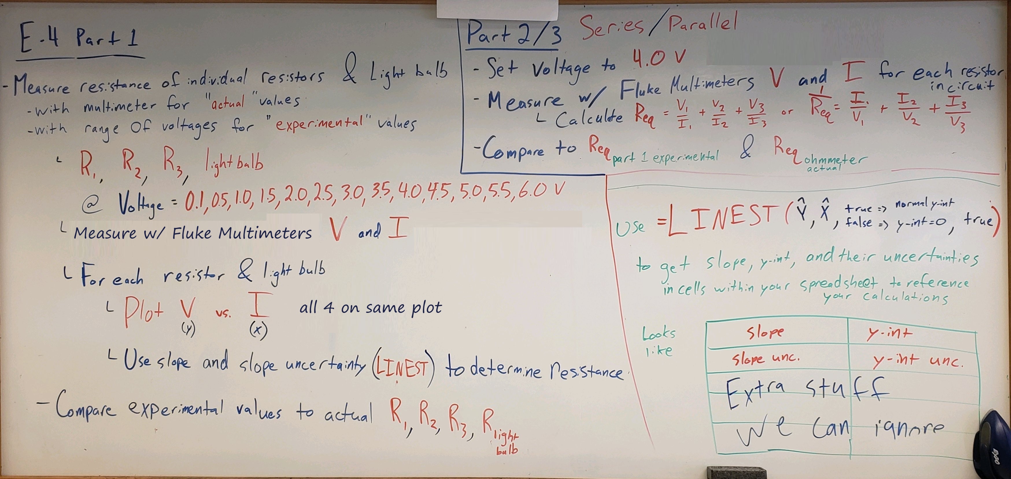
Figure 8:Overview for both main parts of the lab. LINEST() function (use Y,X,True,True).