Error Analysis Review
In laboratory work, it is usually necessary to use experimental apparatus to measure physical quantities. The measurements are seldom, if ever, perfect. As a result, imperfections must be taken into account in any set of physical measurements. One of the most important things to be learned in the laboratory is how to make reliable estimates of the uncertainties involved in any physical measurements and how to handle the propagation of these errors, i.e., to know how the uncertainties affect calculated results of an experiment.
Significant Figures
The number of digits required to express the result of an experimental measurement, so that it reflects the accuracy with which the measurement was made, are known as significant figures. Thus, the number of significant figures reflects the limitation of the measuring device and/or the experimenter. Whether the calculations are performed by hand or on a computer, the number of significant figures displayed in the final result must reflect the limitations of the experimental measurement. Often, a computer program will, by default, display either too many or too few digits. If too few digits are displayed, you need to adjust the program setting to show more digits.
For example, if the length of a cylinder is measured as , this quantity is said to be measured to four significant figures. If written as , we still have only four significant figures. The zeros preceding the “2” are used only to indicate the position of the decimal point. The zero between the “2” and the “6” is a significant figure, but the other zeros are not. If the above measurement is made with a meter stick, the last digit recorded is an estimated figure representing a fractional part of a millimeter division. All recorded data should include the last estimated figure in the result, even though it may be zero. If this measurement had appeared to be exactly 20, it should have been recorded as , since lengths can be estimated by means of this instrument to about . When the measurement is written as it indicates that the value is known to be somewhere between and , whereas the value indicates a range between and . Conversely, retaining too many significant figures implies greater accuracy than the figures actually represent.
Rules for Significant Figures
When deciding the number of significant figures to retain, the following rules apply:
When collecting data, only one estimated figure is retained as a significant figure.
In addition and subtraction, do not carry the result beyond the first column that contains an estimated figure. All figures lying to the right of the last column in which all figures are significant should be dropped.
In multiplication and division, the result should have as many significant figures as the factor with the least number of significant figures.
When dropping figures that are not significant, round to the nearest significant digit. That is to say, the last figure should be unchanged if the first figure dropped is less than 5. The last figure retained should be increased by one if the first figure dropped is 5 or greater.
While performing intermediate calculations, it is safer to carry more significant figures than is required in the final result. You can always fix it when you’re done.
Examples --- Addition & Multiplication
The following examples help illustrate these rules.
Addition
When adding these four numbers:
  427.5
   28.03
    0.0654
  396.0
  ------
  851.6
the result is rounded to the first decimal digit (851.6) because the first term (427.5) in the sum is only given to one decimal digit. The sum is expressed to the proper number of significant figures.
Multiplication
In our next example, we will calculate the area of a rectangle. If its length is measured as and width as , the area as provided by a calculator is
Since each factor has three significant figures (as opposed to the five from the calculator), the result should instead be reported as
Error Analysis Procedure
This section is a guid to performing error analysis for an experiment. Steps for performing error analysis are:
Identify the likely sources of measurement error.
Possible sources --- Instrumentation, experimental setup, procedure
Determine/explain whether errors are systematic or random (see Types of Errors).
Estimate the magnitude of measurement errors using:
Equipment specifications
Significant digits displayed
Your estimate of how accurately you can read the instrument
The range or standard deviation of repeated measurements (see Types of Errors).
Calculate the magnitude of the expected error in calculated quantities due to measurement errors (see Propagation of Systematic Errors through 1. Brute Force & 2. Calculus).
If the difference between your experimental results and the expected results/accepted values is much larger than the expected error, check for:
Experimental procedure mistakes
Calculation or unit conversion errors
Incorrect use of degrees vs. radians
Underestimated measurement error
Incorrect constants or other common values
Report results with the correct number of significant figures (Significant Figures) and the calculated error, otherwise noted as the range or experimental value ± uncertainty.
Types of Errors
Experimental measurements are characterized by precision and accuracy.
A set of measurements is precise if the measurements are closely clustered. (e.g. Figure 1-left)
A set of measurements is accurate if the average value is close to the expected value. (e.g. Figure 1-center)
A set of measurements is both accurate and precise if the measurements are closely clustered close to the expected value. (e.g. Figure 1-right)
Random errors increase scatter and reduce precision. They arise from uncontrollable variations and inherent limitations of the equipment; they can be estimated and reduced by repeated measurements. Systematic errors arise from calibration issues or faulty methods; they can reduce precision and cannot themselves be reduced by repeated measurements. Often you can estimate precision errors by considering the equipment and its specifications.
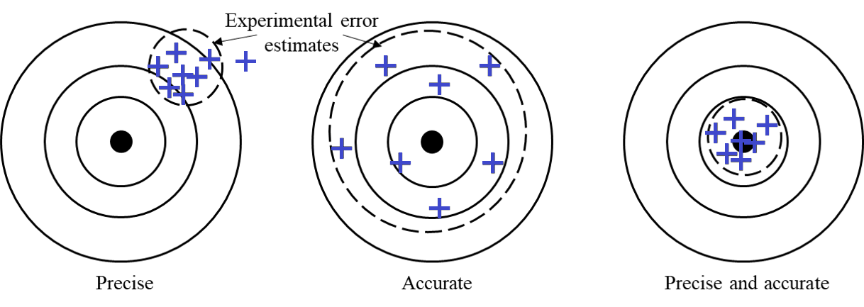
Figure 1:The distinction between precision and accuracy.
Error Propagation of Measurement Uncertainties
Error analysis can help you recognize if your results are consistent with a known or expected value. Each measurement has some combination of systematic and random errors.
Make your best estimate of the measurement uncertainty for each measured value
For direct measurements, think about how confident you are in your measured value. How much could you increase or decrease the measurement tool while still being confident this uncertainty range is still representative of your measurement.
E.g. using a triple-beam balance, you measure , but the level line still appears level when you push the slider to , your value ± measurement uncertainty range could be .
Your estimate may include instrument limitations and variation of measurements over multiple trials. Calculate the differences between your experimental results and any known values.
Recalculate experimental results using maximum and minimum values to determine the expected range of outcomes. Complete this in your spreadsheet by changing your measurements by adding or subtracting the estimated errors. Observe the range of experimental values (maximum and minimum) that you find in these recalculations. If the expected values fall too far outside this range, there is some problem which you need to address.
Example: Error Propagation --- Density of a Block
Suppose you are measuring the density of a rectangular block. The block has dimensions length , width , height , mass each with their respective measurement uncertainty. The calculated density is mass divided by volume.
Given
, ,
Uncertainty in length:
Uncertainty in mass:
The experimental density is
To find the max/min range, the maximum density consistent with your measurements is the ratio of the maximum mass and the minimum volume:
and similarly, the minimum density is . If the expected value lies outside this range, further investigation is required. If the expected density is not in this range, you need to consider possible explanations:
Errors in the measurements could be larger than you estimated
Actual density could be different from the expected value
Your calculation may be wrong
Perhaps the shape is not exactly rectangular
The two types of errors illustrated in Figure 1 require different treatment. The systematic errors illustrated on the target labelled Precise cannot be reduced by taking more measurements, while the average value obtained with the random errors on the target labelled Accurate improves with more measurements. The following sections provide guidance on analyzing systematic and random errors.
Random Errors
Random errors are inherent in nearly all measurements. They arise because of uncontrollable conditions affecting the observer, the measuring device, and the quantity to be measured. On the basis of probability, these errors are as likely to be positive as negative, and more likely to be small than large.
Independent repeated measurements and use of their average in any calculation reduce their effect. This minimization is only achieved if the measurements are independent. A common mistake is biasing a new measurement to agree with the previous measurements. This mistake makes the measurements more precise, but less accurate as shown in Figure 1. Taking truly independent measurements is the best way to reduce random error.
Mean, Standard Deviation, Standard Error
The most well established method to quantify the spread of random errors in a measurement is to compute the standard deviation. Suppose you make measurements of a certain quantity . The average value is:
and the standard deviation of the individual measurements is
In Excel, these operations can be carried out using the functions AVERAGE() and STDEV() or STDEV.S().
If you perform many measurements, then your estimate of the average value improves. The standard deviation of the mean (a.k.a. standard error) for measurements is
Your best estimate of a measurement is then .
Example of Average ± Standard Error
Suppose you take four length measurements (cm): 7.65, 7.61, 7.66, 7.68
The mean value is
and the standard deviation is
The standard error (i.e. standard deviation of the mean) of the average value is thus reduced to and therefore the best estimate of the length is .
Estimation through Variation or Instrumentation
Frequently, a set of measurements has to be taken in an experiment under a prescribed condition. It may be difficult to judge exactly when this condition is satisfied. In this case, it may be necessary to vary the physical quantities that produce this condition and to note how much each may be varied without appreciably altering the prescribed condition. This variation may be used to determine the error.
Finally, the measuring devices (meter stick, voltmeter, and so on) are not perfectly accurate even if one could make a precise reading with them. The manufacturer specifies the accuracy in the measuring device; for example, a particular type of voltmeter may be guaranteed to give readings accurate to of full scale reading. Part of this tolerance is random error that can average out by taking multiple readings. As discussed in the next section, another part of the instrument error is systematic. An ammeter may always read high because of the value of a resistor internal to the device.
Systematic Errors
Systematic errors occur in an experiment because of a defective measuring apparatus, faulty methods, or incomplete working equations or assumptions. They are definite in sign and magnitude and cannot be reduced by averaging because the same error is included in each measurement.
These errors are often more important than the random errors. Calibrating the measuring apparatus, modifying the method, or correcting the equations may reduce them. These are generally described as corrections that are made in the performing of the experiment.
Examples of Systematic Errors
The reading of a Vernier caliper may not be zero when the jaws are in contact. This so-called zero error must be corrected for in using the instrument, i.e., the instrument must be calibrated. Otherwise, all measurements made with the caliper will be in error by a determinate amount, the zero error.
In many experiments time is measured with a stopwatch. Using a stopwatch that does not run at the proper rate would introduce an instrumental systematic error. A watch that ran too fast would cause all times recorded to be too high.
A more significant systematic error encountered with a stopwatch is reaction time error. In measuring the time for an air track glider to travel down an incline, the observer may introduce a systematic error due to the reaction time required to stop the watch and a random error due to variation in reaction time.
Report these sources of error as Vernier caliper error or reaction time error. The expression human error is too ambiguous to be useful in describing measurement errors.
Difference Between Experimental and Expected Values
If the true value of a quantity is known, then the systematic error can be estimated as difference between the experimental and expected values. It is important to remember that this is an estimate of the systematic error. The difference between your experimental value and the expected value is not an estimate of the random experimental error.
To report this difference as a percentage (percent difference), divide the difference by the true, expected, or actual value and multiply by . In Excel, you can use percent format instead of multiplying by .
The percent difference between experimental and actual values is
Sometimes, rather than a difference to actual values, you will be looking at how some quantity changes from an initial to final state. Similar to percent difference, you can report a percent change (when applicable) to help contexualize the process with
Example of % Difference
Suppose a student measures the value of gravity and will compare to the standard accepted value.
Measured value of gravity:
Standard value:
The systematic relative difference, expressed as a percentage, is
It is important to maintain the proper sign of the error as it indicates whether your experimental value was larger or smaller than the actual value (or increased/decreased in the context of % change). There is no definite allowable difference between the experimental and expected values in this course’s experiments. However, all measurements should be made with the greatest care, so as to reduce the error as much as possible.
It should be noted that the percent difference is not an estimate of experimental error. Any measurement has random and systematic errors even if the percent difference happens to be small.
Often, scientists do not know the actual value of the quantity they are measuring and they give their best estimate with error. Comparing the difference between the experimental and actual values with your best estimate of the experimental error (e.g. using standard deviation , standard error , or direct measurement uncertainties ) will help determine if there is a systematic error in your results.
If the difference is less than your estimated random error, then the results are consistent with the expected value.
Having a zero percent difference could be the result of a lucky cancellation of errors and still just means the results are consistent.
If the difference is significantly more than the estimated error, then you can begin to ask why your result is not consistent with the expected value.
Propagation of Systematic Errors through 1. Brute Force & 2. Calculus
Through indirect measurement, the effect of systematic errors can be followed through the equations used. Two simple examples will be discussed.
Calculation from a Single, Direct Measurement (Sphere)
Consider the volume of a sphere as calculated from a direct measurement of its diameter, . We would use
where . Suppose the value of is measured as and computed to be . It is later discovered that the value of has a systematic error , (unnecessarily large, in all probability). What is the error in and the corrected value of ?
1. Direct, brute-force method
Correct to
Re-compute as
The systematic error in is then or
2. Method based on calculus
Find the derivative of with respect to ,
Note that this shows a direct dependence of a change in on an infinitesimal change in . Now divide through by
If a finite change in , such as the systematic error , is small compared to , then and can be approximated by and , respectively, and so the following can be written:
This means that the fractional or percent error in is very nearly 3 times as large as that in . Another way to say, a 1% error in diameter produces a 3% error in volume. Therefore,
Hence,
and
Calculation from Two or More Direct Measurements (Cylinder)
Consider the volume of a right, circular cylinder as calculated from its diameter and length . For convenience, let be measured as and as . Then,
If has an error of and an error of , what is the error in and what is the corrected value of ?
1. Direct, brute-force method
To obtain
Subtract from
Add to
Recompute as , whereby must be .
2. Method based on calculus
Find the partial derivatives of
so that
Now dividing through by
This shows how fractional errors in each measured quantity contribute to the total error in the calculated result; i.e. the fractional (or percent) systematic error in is very nearly equal to the fractional systematic error in plus twice the fractional error in . In our case,
and
so that
Thus , i.e. the systematic error, is ; the correction is and .