Equipotential & Electric Field Mapping
Background
● Background Overview
Electric fields are a convenient construct to analyze the electrical force between two charges. It is defined as the force per unit charge experienced by one charged body in the presence of one or more other charged bodies. The direction of the electric field is in the direction of the net electric force experienced by a positive charge (e.g. positive to negative). It is illustrative to represent the electric field distribution by lines that continuously point in the direction of the electric field (see solid lines in Figure 1).
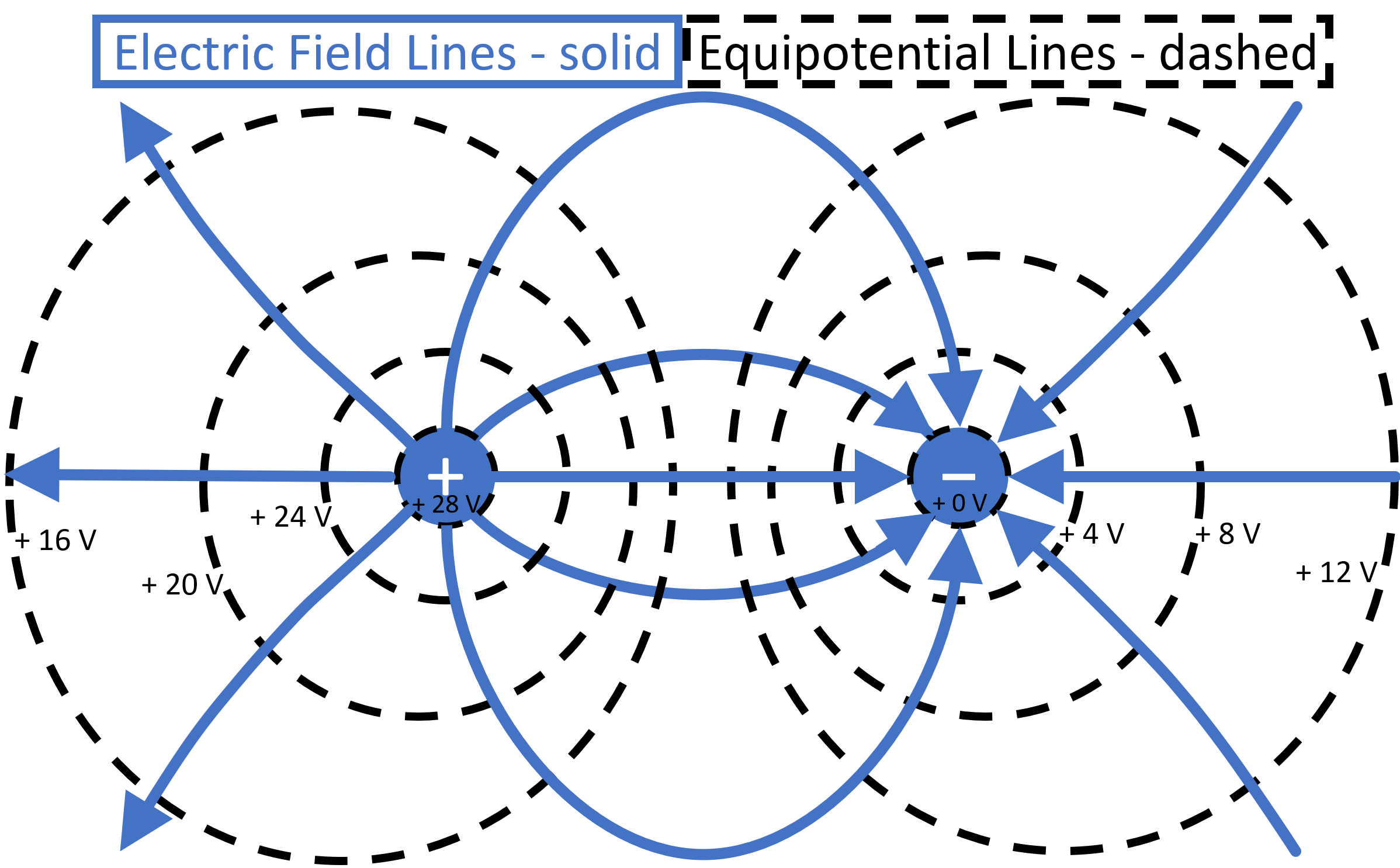
Figure 1:Right) Equipotential (dashed) and E-field lines (solid) between two equal but opposite charges.
The amount of work required to move a unit charge between two points in an electric field is equal to the electrical potential energy difference between the points. The potential difference (voltage), (see dashed lines in Figure 1 relative to ), is defined as the electrical potential energy difference per unit charge between the two points (see charges A and B in Figure 2).
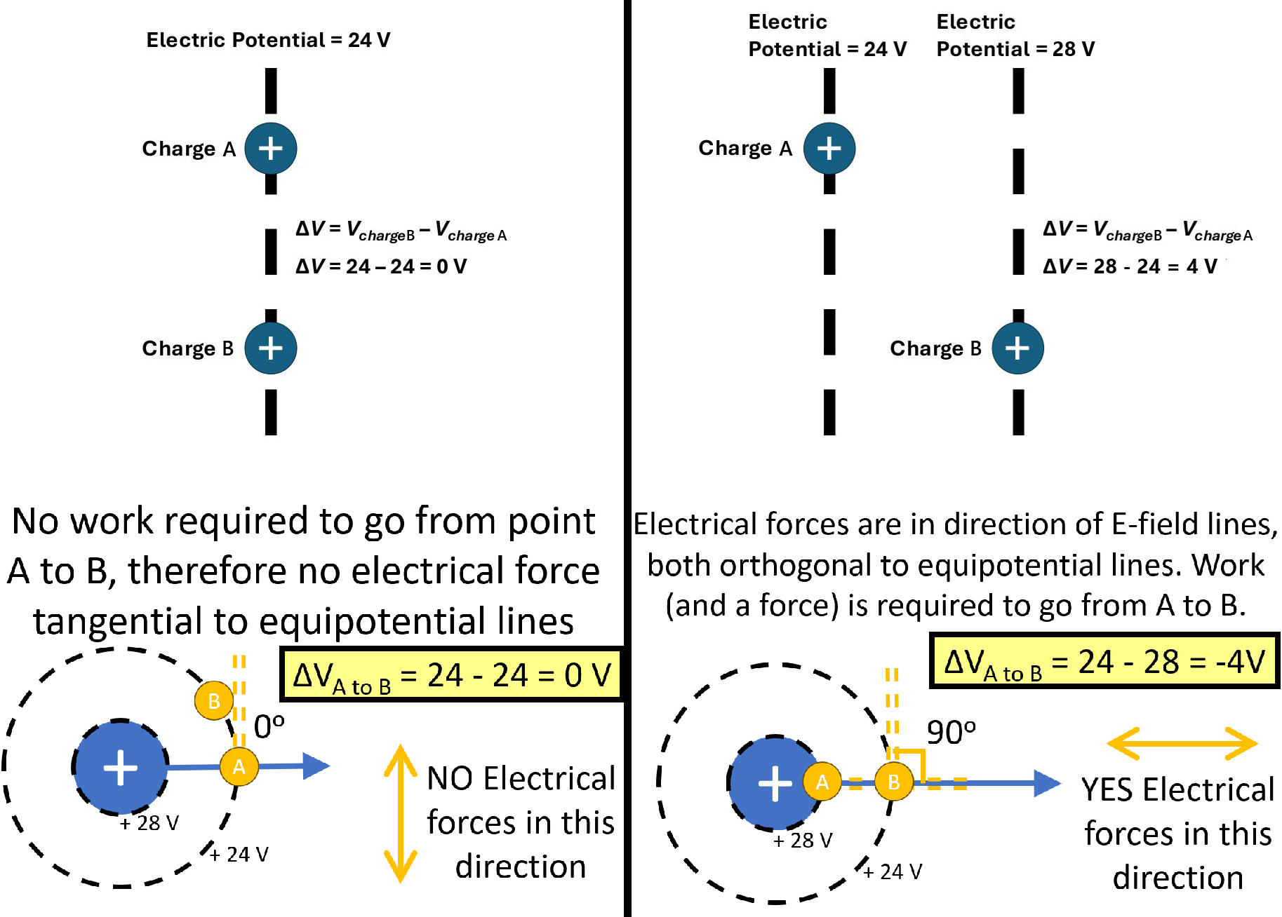
Figure 2:Top-Left) Charges on same equipotential line, no voltage difference. Bottom-left) No work, no forces, along equipotential lines. Top-Right) Charges on different equipotential lines, some voltage difference. Bottom-right) Work can be done, electrical forces in direction of E-field lines.
If the potential difference between two points is zero, the two points are said to lie on the same equipotential line or surface (see Figure 2 left). No work is required to move a charge along an equipotential line or surface. Since no work is done, there cannot be any electric force acting tangentially to the line or surface. Therefore, the electric field cannot have a component parallel (or tangential) to the equipotential line or surface and must instead be perpendicular to it at every point.
Since the electric field is always perpendicular to equipotentials, moving in the direction of the electric field will end up taking you from one equipotential to another. When the potential difference between two points is non-zero, they lie on different equipotentials (see Figure 2 right), and work is required to move a charge between them.
Because a charge at any point experiences a single, well-defined net electric force, the electric field at that point has a unique direction. Therefore, two electric field lines can never cross. If they did, the field would have two different directions at the same location (Figure 3 left). Equipotential lines also cannot intersect, since they must always be perpendicular to the electric field (Figure 4 top).
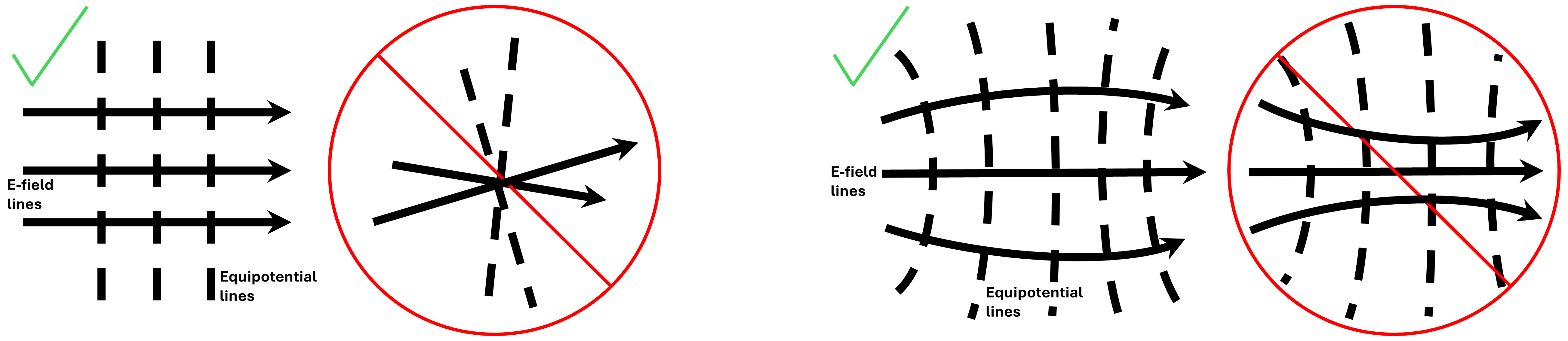
Figure 3:Left) Equipotentials parallel, then E-field lines are parallel. Must not cross. Right) Equipotentials curve away, then E-field lines must curve away (diverge) as well. Must not cross and converge/diverge oppositely.
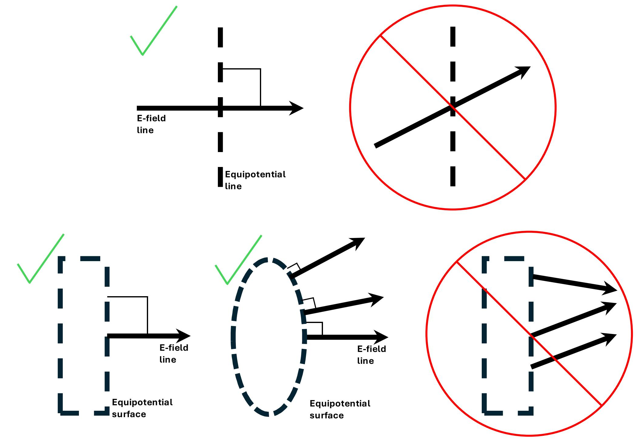
Figure 4:Top) Equipotential and E-field lines always cross perpendicularly. Bottom) E-field lines must leave an equipotential surface perpendicularly as well.
Conductors, like our electrode patterns today, are themselves equipotential surfaces. Therefore, the electric field at the surface of an electrode must be perpendicular to the electrode’s surface (Figure 4 bottom).
If equipotential lines are parallel, the electric field lines must also be parallel. If the equipotentials are curved, the electric field lines will converge or diverge as they pass through them (Figure 3 right). Where field lines converge, the magnitude of the electric field increases; where they diverge, the field strength decreases. As neighboring equipotential surfaces get closer together, they necessarily become more nearly parallel. Consequently, the shapes of electrodes and the spacing between them determine the patterns of both the equipotential surfaces and the electric field lines.
● Experimental Overview
In this experiment, we will qualitatively establish electric field distribution between various pairs of electrodes on a sheet of conducting paper (see Figure 5). With a voltmeter (wiring shown in Figure 5 top), we will measure the potential difference between points on the paper. By plotting lines whose points are at the same potential (i.e. zero potential difference between any two points, or points at the same voltage), we can map out a number of equipotential lines. Note that in three dimensional space, equipotentials are surfaces perpendicular to the electric field. On the two dimensional conducting sheets, equipotentials form lines perpendicular to the electric field. Since we know that electrical field lines must be perpendicular to the equipotential lines, we can sketch a representative family of electrical field lines using the conventions discussed above.
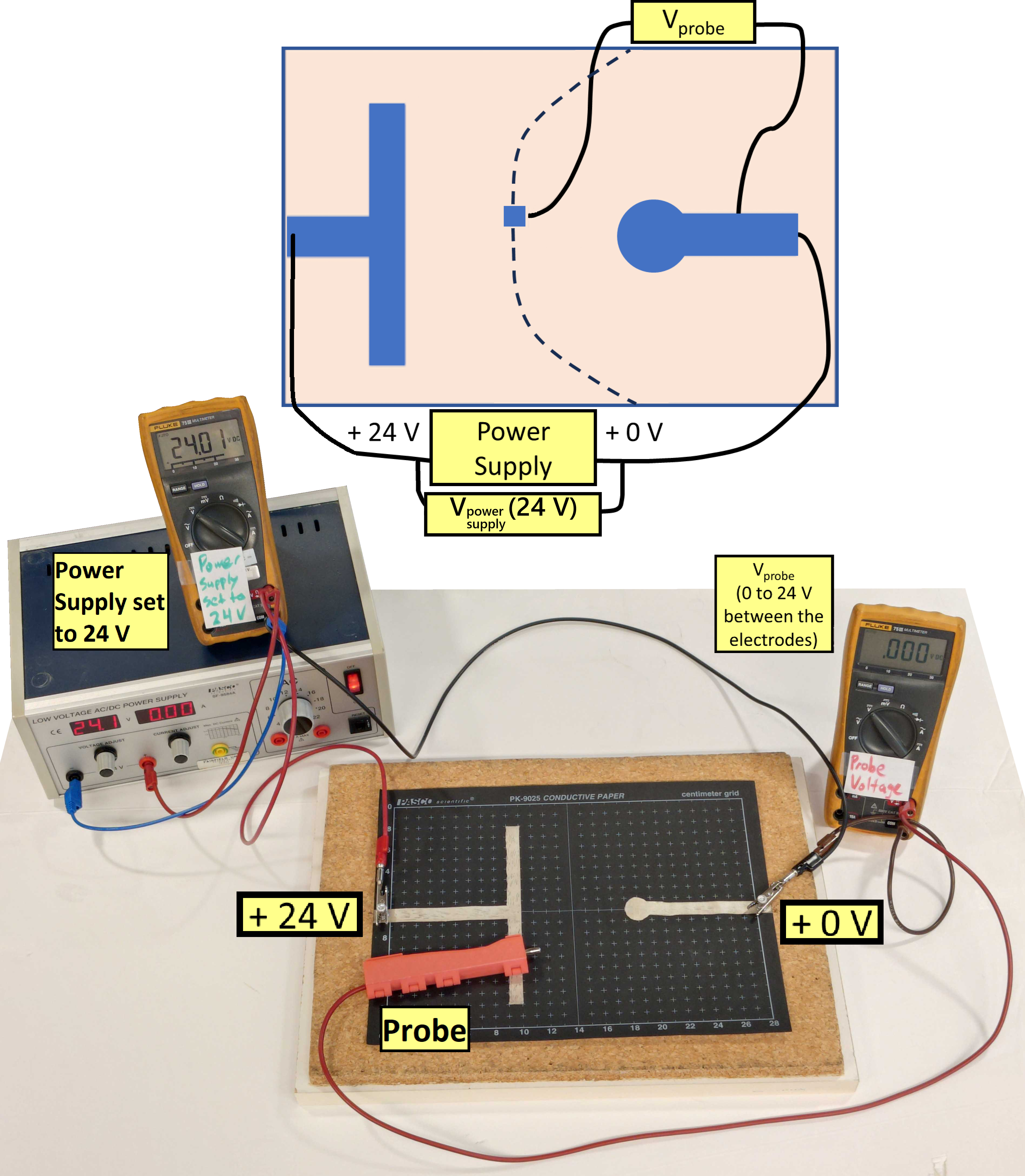
Figure 5:Experimental setup. Top) Schematic example. Bottom) general setup with all parts included, currently set to (white paper for drawing on not shown).
An example of an electrode configuration is illustrated in Figure 5 top. The dashed line indicates a possible equipotential line. In this example, it is specified by the positions on the paper whose potential with respect to the negative terminal of the power supply is . Moving the probe on the paper to other points where the voltage is informs us of the equipotential line location. Since each point on the line is at the same potential, this is one of an infinite number of equipotential lines generated by this electrode configuration. The actual plotting (recording) of the equipotential lines and the sketching of the electric field lines is done on a separate graph paper whose coordinates match the conducting paper with its electrodes.
If we determine a number of equipotential lines for this electrode pattern, we might get the pattern of ‘dashed’ equipotential lines shown in Figure 6. Recall that the electrodes are also equipotential lines/surfaces. Now we can sketch in a representative pattern of electric field lines. Like the equipotential lines, there are an infinite number of possible field lines. We know that the electric field lines begin on the positive electrode and end on the negative electrode; also, they are normal (perpendicular) to all equipotential lines they cross without crossing other E-field lines. A few small arrowheads along the field line indicate the direction of the field. The field lines will be shown as solid lines to clearly distinguish them from the equipotential lines.
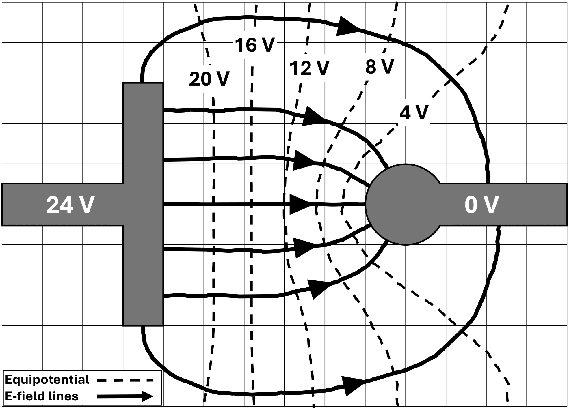
Figure 6:Electric Field and Equipotential patterns drawn from edge to edge of the paper.
Since the direction of the electric force on a test charge is always positive-to-negative by convention, the arrowhead direction of the field lines must be the same. For this example, we start with more or less evenly spaced starting points at the positive electrode. Consider a single field line leaving one of these points. It leaves normal (perpendicular) to the surface. As it approaches the first equipotential surface, the direction of the field line needs to be smoothly adjusted so it crosses it perpendicularly. Continuing to the next equipotential line, the direction of the electric field line is continually and smoothly adjusted to cross this equipotential perpendicularly. Continuing in this manner, the field line is sketched all the way to the negative electrode where it must end on the electrode perpendicular to the local surface.
The electric field lines can be sketched most easily when there are a sufficient number of more or less equally spaced equipotential lines to guide the direction of the field lines. The number of electric field lines that are drawn should be sufficient to clearly show the characteristics of the pattern. The electric field lines should be evenly spaced along the surface of the positive electrode so the density of the field lines in the pattern will show the relative intensity of the electric field. In this pattern you can see the higher concentration of field lines as they approach the smaller radius surface of the right electrode. The same thing would occur at the sharp corners of the left electrode if we happened to start our sketching from a uniform spacing of field lines on the right electrode.
The drawing of both dashed equipotentials and solid E-field lines will be assisted by the use of a “French curve” as seen in Figure 7 and whose use is described in Demo Video: Setup, Procedure, & French Curves. The configurations you will characterize today are shown later in Figure 8 which also includes seven starting positions on the left electrodes to initiate E-field lines (roughly equally spaced).
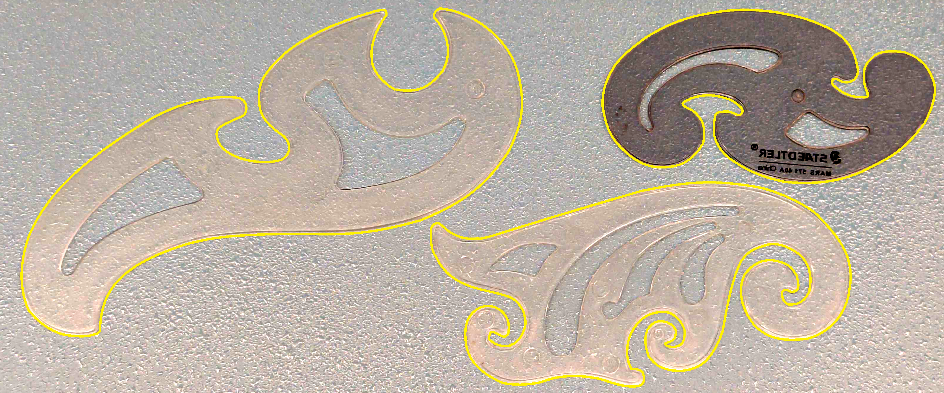
Figure 7:French curves that will be available for interpolating equipotential and E-field lines.
● Equipment
Depicted in Figure 5 and Figure 8.
Low voltage DC power supply,
Two Fluke multimeters -- set to read DC voltage (one for power supply, one for probe)
Folder with three sheets of black conductive paper with different electrode configurations (see Figure 8)
White photocopy of the same configurations for drawing/plotting will be at front table
Cork board with 2 metal push pins (for electrical connection to conductive ink and paper)
x5 Banana plug wires (18 AWG: x3 1’, x1 2’, x1 3’), connecting power supply to voltmeters and electrodes (via alligator clips) on conductive paper
x1 Banana plug wire (18 AWG: x1 3’), in the red holder as the probe wire to determine patterns of equipotential lines
French curves for interpolating equipotential lines and drawing curved E-field lines perpendicular to the equipotential lines determined with the probe
Demo Video: Setup, Procedure, & French Curves
Demonstration video. Reviews overall setup and procedure. *No audio*
If embedding is broken, follow: https://
Experimental Procedure
● Procedure Preview
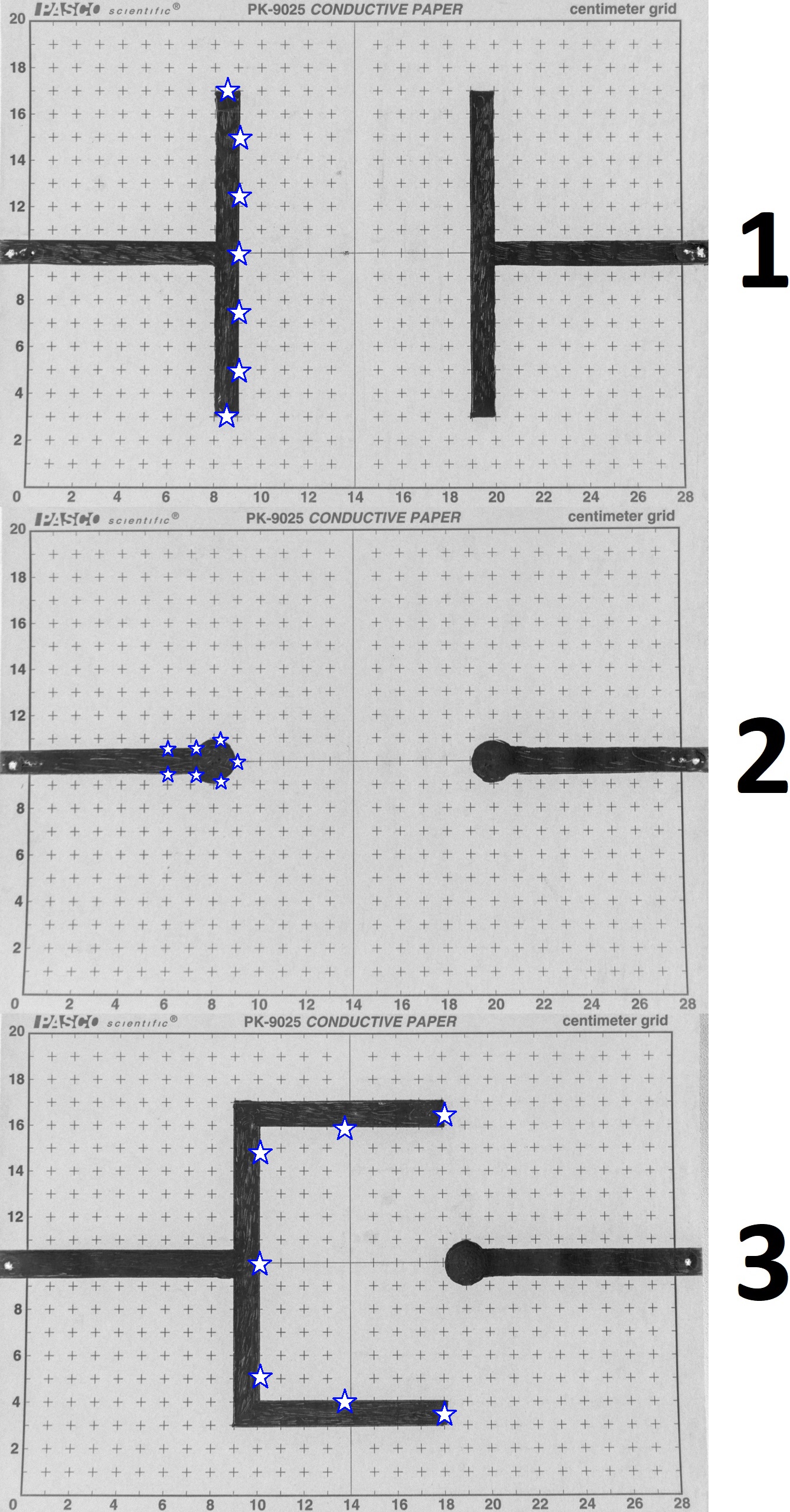
Figure 8:Electrode configurations. The stars show minimum required starting positions for E-field lines.
● Preliminary Setup
Each group will characterize all three electrode configurations (see Figure 8); each person will draw and finalize at least one configuration. Begin with electrode configuration #1. Place a conducting electrode sheet on the cork mounting board and fasten down with a metal push pin at the end of the silver electrodes. Make sure the pins are pushed all the way down to make electrical contact with the electrode.
Refer to Figure 5 to set up electrical connections. They should already be accurate, but use the following to confirm or perform connections if necessary.
Connect both the positive (red) terminal of the first power-supply voltmeter and the left-hand electrode to the positive (red) terminal of the power supply.
Connect the right-hand electrode similarly to the negative (black) terminals of both the power supply and power-supply voltmeter.
The probe (red) will be connected to the positive (red) terminal of the second probe voltmeter, while the negative (black) terminal of the probe voltmeter is connected to the right-hand electrode.
A photocopy of the electrodes on a sheet of graph paper are provided for each of the electrode configurations at the front table. They will be used to record the points of the equipotential lines determined in the following steps.
Turn on the power supply and set the voltage to , confirming with the power-supply voltmeter. Gently place the probe on the positive electrode and adjust the power supply so the probe voltmeter reads . Check that the probe is making electrical contact by moving it, with a very light downward pressure, from the positive electrode to the negative electrode. Verify that the voltage decreases smoothly from .
● Equipotential Mapping
With a very light downward pressure, move the probe along one of the long sides of the conducting paper until the voltage on the probe voltmeter is . Mark the point on the graph paper.
Now move the probe about a centimeter away to find the next nearest point as close to as possible and mark it on the graph paper. After having two positions marked, you can start to indicate the direction of the equipotential. The tangent to the equipotential will help you search for the next point. Move again and mark the next point and direction on the corresponding point on the graph paper copy. Continue in this manner until you reach the opposite side of the conductive paper. If it appears that the equipotential line is curving rapidly, as it might near a small radius edge of an electrode, it will be helpful to take more closely spaced points.
With the aide of a French curve (reviewed in Demo Video: Setup, Procedure, & French Curves), draw a DASHED CURVE through these points and tangent to the equipotential which can be defined as the equipotential line. These points must be connected by a carefully drawn, smooth curve, making sure they do not cross other equipotential lines, including the surface of the electrodes.
Now, move the probe along the edge and find a point. Proceed to find and plot the series of points of the equipotential line from one edge to the other of the conductive paper.
Proceed in this fashion in steps and plot the rest of the five equipotential lines between the electrodes, and label all 7 equipotentials (). Note: The electrode surfaces represent the zero and equipotential lines. Add additional equipotential lines as needed to ensure full characterization of the equipotential space across the page.
● Electric Field Lines
After the equipotential lines have been determined, draw in the corresponding electric field lines starting at one electrode and running to the other electrode.
Use a French curve and the technique described in the demo video, Demo Video: Setup, Procedure, & French Curves.
Sketch in at least seven SOLID lines to give a representative picture of what the electric field looks like (minimum 7, equally spaced starting positions are indicated by ★ in Figure 8 and reiterated in Figure 9). Add additional E-field lines as needed to ensure full characterization of the electric field including lines that may go off the page. Sketch lines including the areas at the edges of the paper.
Recall that the electric field lines do not cross and are perpendicular to the equipotential lines, including the electrode surface edges (reminders: Figure 4, Figure 3, Figure 6). Compare them with similar figures in the manual and if they are not satisfactory, then take additional data as necessary.
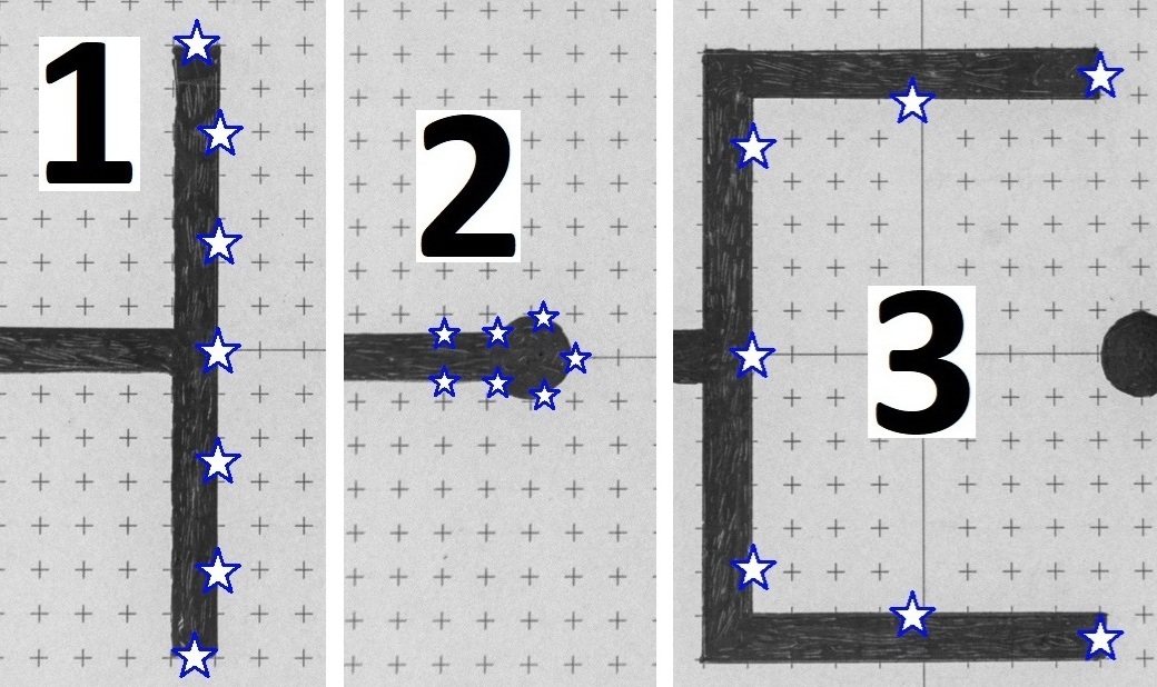
Figure 9:Electrode configurations. The stars show minimum required starting positions for E-field lines.
These field patterns should be carefully and neatly reproduced, on each graph paper with the corresponding electrode pattern. As with any graph or illustration, they must be clearly annotated with appropriate labels, potentials, polarities, and field directions. ALSO, INCLUDE THE PLOT-DRAWER’S NAME AND GROUPMATES’ NAMES ON EACH PLOT.
Repeat from Step 1 for each electrode configuration.
When you are finished with all three electrode cases, reset your experimental setup before leaving and ensure your sketches are complete.
Post-Lab Submission --- Interpretation of Results
Note: For this lab, your results will be very qualitative.
● Finalized “Spreadsheets”
Make sure to submit all three of your finalized field mappings.
INCLUDE THE PLOT-DRAWER’S NAME AND GROUPMATES’ NAMES ON EACH PLOT.
Include all labels and markings as described throughout the procedure.
Submit to the “spreadsheets” assignment in Blackboard.
● Post-lab Writeup
In a paragraph, summarize your error analysis. Be qualitative, and quantitative when meaningful.
What are possible sources of systematic (i.e. affecting accuracy) and random (i.e. affecting precision) errors?
How could you increase your confidence (i.e. decrease you uncertainty) in your electric field lines (i.e. final results) considering your methodology from today’s lab? Consider electrode configuration 3 (Figure 8 3).
In a paragraph, summarize the results you have determined in each case. Consider:
What was the point of today’s lab; what did we aim to discover?
How do the equipotential lines that you drew physically relate to the electrode spacing and shapes?
How do the E-field lines that you drew physically relate to both the electrode and the equipotential patterns? -- What happens to your E-field lines when equipotentials were curved, or closer together/further apart?
If you placed an electron on an equipotential, say the equipotential, what direction would the electron move?
What do the electric field and electric potential patterns in electrode configuration 1 (Figure 8 1) suggest about the electric field between the two plates in lab E-1?
The Whiteboard
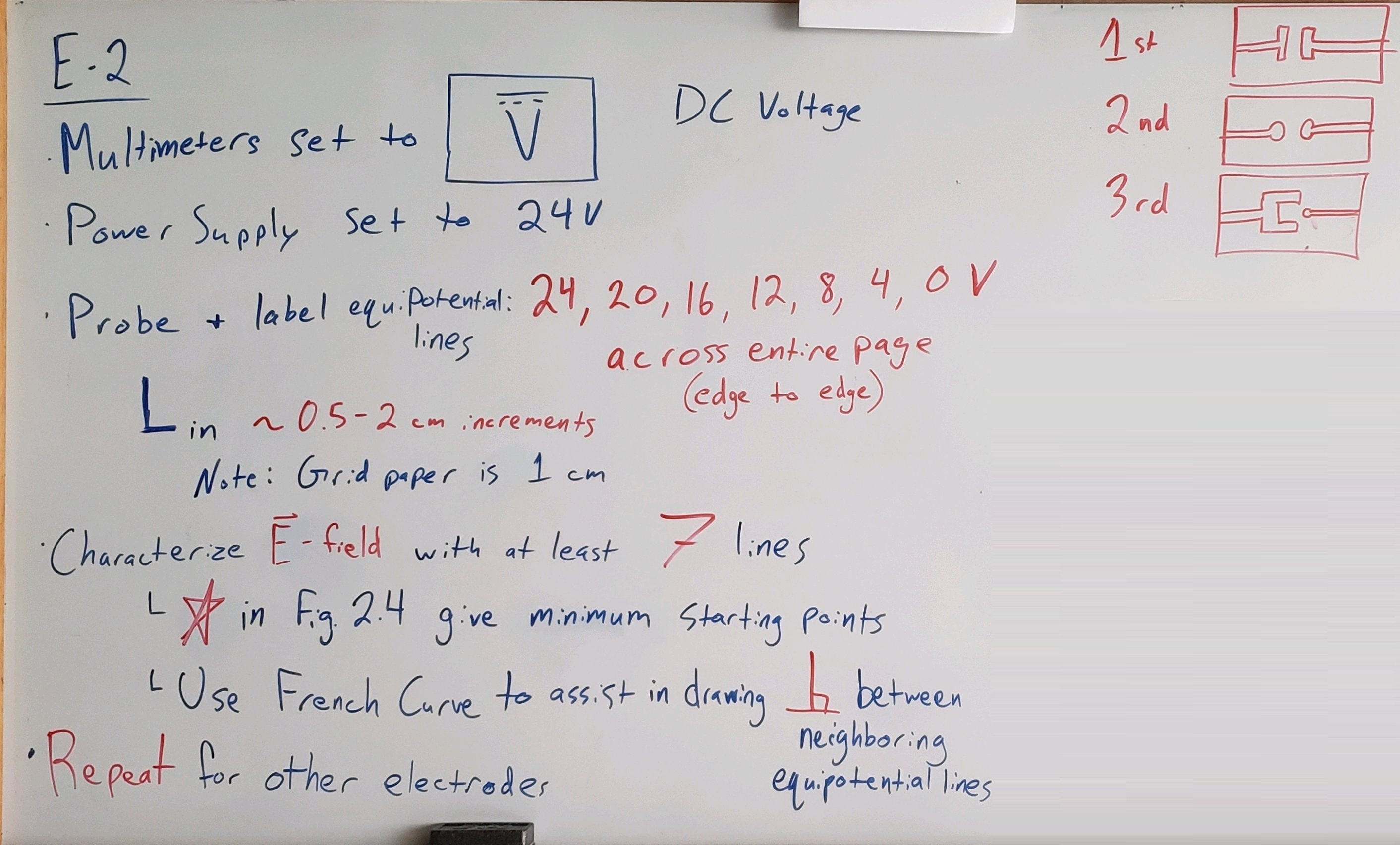
Figure 10:Overview.