Magnetic Force & the Determination of μ₀
Background
● Background Overview
By measuring the magnetic force between two parallel current-carrying conductors, the permeability of free space, , will be experimentally determined. is a fundamental constant of nature, and, with its electric equivalent that we determined in an earlier experiment, we will now be able to determine the magnitude of the velocity of propagation of an electromagnetic wave --- the speed of light. These constants are related to the speed of light, c, by the following relation, derived from Maxwell’s equations which describe the behavior of electric and magnetic fields:
You will measure here, and, with your previous measurement of , determine the speed of light .
The 2019 redefinition of SI units defined exact values of fundamental constants including the electron charge , the speed of light , and Planck’s constant . The second is defined in terms of the frequency of a Cesium atomic clock. As a result, the value of , the magnetic constant, must now be experimentally determined.
Note: Until 2019, was defined to be exactly T⋅m/A. This 2019 value is so close to the current best measurement, that you can use T⋅m/A as the accepted value.
The magnetic field strength a distance from the center of a very long, straight conductor carrying a current is given by:
A conductor of length [m] carrying a current [A] in a magnetic field of strength [T] experiences a force [N], given by:
where is the angle between the vectors and . If the magnetic field is produced by the current in a second conductor, the currents in the two conductors exert equal magnitude and opposite forces on each other.
For the case of two long, parallel conductors, each carrying the same current and separated, center-to-center, by the distance , the force between the two conductors is the force on one in the magnetic field of the second. Thus if (2) is used in (3), we obtain for the force:
By measuring the force between two such conductors, the value of can be determined. By considering the parameters of the apparatus to be used, it can be seen that the magnitude of the force between the two conductors is quite small and will require some care to accurately measure. If is about 30 cm, about 10 A, and about 2 mm, the force would be in the range of 10-4 N, or the weight of a few milligrams of mass. Since this force is well below the weight of a reasonable conductor to be used for the experiment, a counter weighted balance system will be used to provide the mechanical support for the movable conductor. This is essentially the same apparatus as Electric Force & ε₀ Lab. The movable conductor can then be loaded by a known mass whose weight can then be matched by the small magnetic force. The apparatus is schematically illustrated from a top-down perspective in Figure 1.
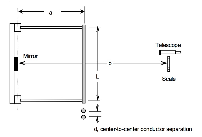
Figure 1:Apparatus dimensions from a top-down perspective, similar to the apparatus setup from Electric Force & the Determination of ε₀.
As before, similar to the setup and measurement methods from the Electric Force & ε₀ Lab, an optical lever, telescope and scale are used to observe the deflection of the balance, which carries the movable, upper conductor. The magnitude of the magnetic force can be measured when the magnetic force has restored the loaded system to its original position. In this case we make the same magnitude current flow in opposite directions in the two conductors so the force between the two conductors is repulsive. Thus on the upper conductor, there is a gravitational force down (the weight of the applied mass) and a magnetic force upward which we will adjust by controlling the current equal to the gravitational force. More conveniently than the electric force version of the balance beam, this equilibrium is stable!
With the required balancing current determined along with the other dimensions of the apparatus, we can now determine the value of .
● Equipment
Table 1:Equipment
| Category | Items |
|---|---|
| Optical Measurement | • Telescope with crosshair • Centimeter-scale ruler mounted on vertical pole |
| Power Supply | • AC power from wall outlet controlled by large cylindrical transformer/potentiometer (0–100% of wall power, ~0–20 A) Dial markings are not accurate; ignore scale on knob • Voltage transformer (small metal cube) reducing AC voltage to ~6 V |
| Current Measurement | • Fluke multimeter used as AC ammeter (,  ), connected in series with circuit ), connected in series with circuit• One lead in 10 A port  , other lead to COM port , other lead to COM port  |
| Masses & Tools | • Small masses (5, 20, 50, 100, 200 mg) • Plastic tweezers for handling masses |
| Parallel-Conductor Apparatus | • Bottom conductor fixed in place • Top conductor free to swing vertically when current or mass changes • Adjust so conductors are parallel when 0 mg is applied • Mirror used with telescope to read ruler and determine balance beam angle • Beam lift knobs to reset top conductor position • Leveling screws to level apparatus |
| Electrical Connections | • 4x banana plug wires (12 AWG) • 2x 1 ft • 2x 3 ft • Connect transformer ammeter parallel-conductor apparatus |
| Additional Equipment | • Protective box with mirror-to-scale distance written on it |
● Adjustment of apparatus
The apparatus has been carefully adjusted before your lab and should not require further significant adjustments. This section describes how the apparatus was prepared. If something seems to need adjusting, see the lab instructor. The apparatus is very similar to the apparatus setup from Electric Force & ε₀ Lab.
The beam lift provides a definite location for the beam and thus guarantees continued alignment of the parallel conductors. Use the beam lift each time you change weights or relocate the counterweight.
The fixed conductor can be adjusted vertically, the movable conductor horizontally, so that the conductors are parallel. If the conductors are NOT parallel with no mass in place, seek the instructor’s help.
The counterweight behind the mirror can be used to change the equilibrium separation of the conductors.
Level the apparatus with the adjusting screws so that it sits securely on the table.
Mirror-to-scale distance was measured from rear of mirror (reflective surface) to roughly the middle of and on the scale (ruler).
Demo Video: Setup & Procedure
Some clarifications, additions, or corrections since this video is slightly outdated:
Wires are thicker and safer now, still don’t touch, don’t exceed 20 A
White board slightly outdated as there have been slight changes
Masses in decreasing order, rather than increasing order
Using average and uncertainty (not standard deviation)
Speed of light just from plotting-derived (i.e. from
LINEST) values from first lab () and today’s lab ()
Demonstration video. Reviews overall setup and procedure. *Yes audio*
If embedding is broken, follow: https://
Experimental Procedure
● PRECAUTIONS
The wire frame that supports the current carrying conductor and counterweight is supported on knife edges. The frame is easily bent, and the knife edges can be easily damaged. Treat the system with the same care as a precise analytical balance. Handle the weights with tweezers and store them in the case.
The current must pass through the knife edges and intense local heating is produced. Reduce the current to zero as soon as possible after making the observations.
● Preview
● Preliminary Setup
If is the mirror-to-scale distance and is the length of the frame (see Figure 1), then a straightforward geometrical analysis (like in Electric Force & ε₀ Lab) will show that the vertical displacement of the conductor, , is given by:
where is the change in scale reading from the equilibrium value and the value when the two conductors are in contact (the contact reading is determined by adding a mass to the pan which depresses the beam until contact occurs). The factor of 2 results from the fact that the optical path reflected off of the mirror to the scale rotates through an angle twice that of the beam holding the movable conductor.
However, the change in scale reading doesn’t account for the conductors’ thickness. Since the B-field generated by current flowing in the cylindrical conductors is organized about their center, we must add in two radii to get the center-center separation between the two conductors. This gives us:
where is the radius of the conductor (multiplied by two to deal with the fact that we’re dealing with two conductors).
Investigate the use of the telescope and scale so that the rotation of the frame can be measured in terms of scale divisions (see Figure 2).
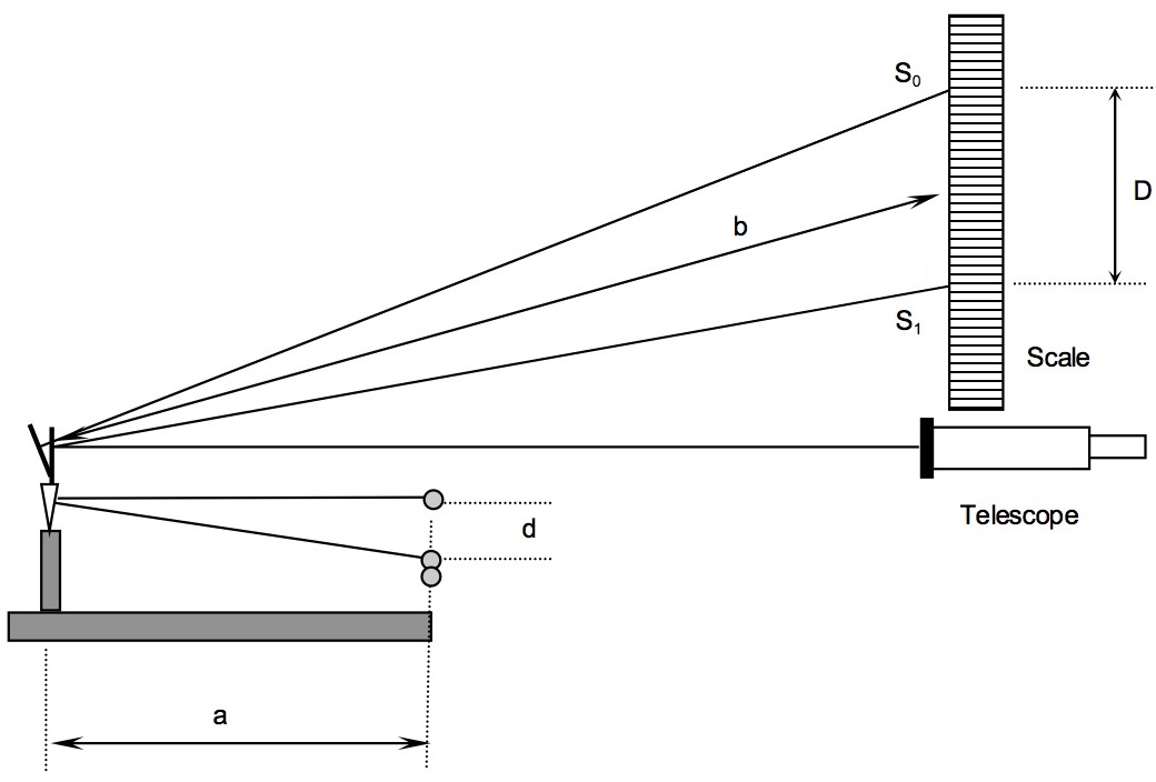
Figure 2:Schematic of the measuring apparatus, similar to the setup and measurement methods from Electric Force & ε₀ Lab.
Do not turn on the power supply until requested in the procedure later in ● Experimental Data Collection.
Create a common data table with:
: length of frame,
: mirror-to-scale distance (on top of protective box)
: wire/bar length
: wire radius
: equilibrium crosshair position
: bars touching crosshair position
: ruler (a.k.a. scale) distance between and
: length of frame
: acceleration due to gravity for Fairfield, CT,
: accepted value of the permeability of free space,
: accepted value of the speed of light,
Also add in the plotting-derived (i.e. from
LINEST) from the first lab for each member of your lab groupOf your group members’ values, take the average (), and use the standard deviation () of your groups’ values as the uncertainty for later speed of light use.
If you are completing the lab individually, use your single plotting-derived and its associated uncertainty
In order to measure the equilibrium separation distance, , of the conductors, two readings are made.
The first is the scale reading, , at the equilibrium position, i.e. when no mass has been applied to the pan on the movable conductor.
The second scale reading, , is made when the top conductor contacts the lower conductor (Figure 2). Place a sufficient mass in the pan on the top conductor to make it contact the lower, stationary conductor. Record .
⚠️ POWER MUST BE OFF FOR THIS STEP ⚠️
You will periodically verify that and are not changed throughout the experiment.
Determine from two scale readings (reminders: absolute value there is to represent the total distance between and . If your crosshair crosses 0, make sure to consider the negative).
Calculate and record the conductor separation distance, . Refer to Figure 1, Figure 2, (6).
Prepare a data table with columns for the variables below. You’ll have rows for each trial as well as for averages. Reminder, you will conduct 27 trials total by conducting three rounds of sequentially changing the applied masses:
Trial number
Lab member’s initials (person looking through telescope)
: Applied mass
: Applied magnetic force What does this equal?
: Minimum current required to return to the equilibrium position
: Maximum current required to return to the equilibrium position
: Current required to return to the equilibrium position
: Estimated current uncertainty (to be assumed as majority source of uncertainty for today)
: Current squared
: Current squared
: Experimental value of
: Maximized experimental value based on
: Uncertainty in experimental value
: Magntitude of difference between experimental and accepted values of
● Experimental Data Collection
With the power off 🟥, make sure the conductor beam is still at equilibrium, then place the current trial’s mass on the upper conductor (see full list in Table 2). The top bar will swing downwards. In following steps, you will apply a current to counteract the gravitational force. Record the trial’s mass value and calculate (reminder, use SI units; these masses are in units of milligrams; hint: what does the magnetic force balance?).
Table 2:Experimental Trials Breakdown
Student on telescope Trial Applied Masses (mg) POWER ON 🟢 / Off 🟥 Student #1 200, 175, 150, 125, 100, 75, 50, 25 ON 🟢 Student #1 (and #2) 0 (ensure has not changed) Off 🟥 Student #2 200, 175, 150, 125, 100, 75, 50, 25 ON 🟢 Student #2 (and #3) 0 (ensure has not changed) Off 🟥 Student #3 (or #1
again for a group of two)200, 175, 150, 125, 100, 75, 50, 25 ON 🟢 Student #3 (and #1) 0 (ensure has not changed) Off 🟥 Calculate (hint: what does this equal?) and determine current required to balance the weight of the applied mass and return to equilibrium by finding a current range. Make sure the transformer setting is zero before turning on the power. Turn on 🟢 the power supply and slowly increase the current until the bars return to parallel (i.e. crosshair in telescope back to , as it was with no applied mass on the top). Determine this by having an observer watching the scale reading with the telescope during this process. The telescope observer should be calling out instructions to the power supply operator to slowly approach the value.
When the value is approximately reached, call out to the power supply operator.
Power supply operator shall decrease the current until the telescope observer is no longer confident the crosshair is at the position, at which point the telescope observer shall call for a minimum current reading from the multimeter and record the lower end of the range of current .
Power supply operator shall then increase the current until the telescope observer is no longer confident the crosshair is at the position, at which point the telescope observer shall call for a maximum current reading from the multimeter and record the upper end of the range of current .
As soon as you make these readings, reduce the transformer setting to zero and turn off 🟥 the power switch. Under no circumstances should the current exceed 20 A.
Calculate applied current as the average of the min and max currents,
Calculate applied current uncertainty as half the difference between max and min current,
Calculate as well as by maximizing and taking the difference (i.e. )
For the current trial, calculate from (4) and determine its uncertainty by maximizing by your measurement uncertainties (primarily due to current today) and taking the difference (i.e. , hint: should be a positive value).
Also calculate the difference between your experimental and accepted permeability of free space values for quick comparisons.
With power off, replace the applied mass for the next trial, and repeat the previous steps in ● Experimental Data Collection to find the current required to balance the system again, and subsequently calculate again.
● Data Analysis
○ Averages
Calculate your average values from everyone’s trials (ignoring those that give a divide-by-zero error):
Average experimental value
Average experimental uncertainty
, the average difference between experimental and accepted
If, after performing the graphical data analysis below, you find some or all of the data unacceptable, repeat from Step 4, checking that the telescope and scale were not disturbed during your measurements.
○ Graphical
The graphical display of data permits the comparison of all the values and associated errors at once. Points that depart markedly from the general trend of the data are quickly detected. We expect from theory (4) that magnetic force and current are related like:
Using all of your data points from all rounds and trials, including those at equilibrium () that you should have ignored earlier when you calculated for each individual trial and the overall average:
A) SCATTER PLOT 1 --- vs. (i.e. as ordinate () and as abscissa ()). Fit a trend line through the all these points, display the trendline equation on the chart, and confirm the slope of the line matches what you found with the
LINEST()function (for review, see Plotting in Excel). From (4) and (7), the slope value of is given by (8).Calculate the plotting or slope-derived by rearranging (8) and using this experimentally determined value .
Similar to earlier, calculate by maximizing by the slope uncertainty (output from the
LINEST()function, Plotting in Excel), and subsequently taking the difference:Also calculate the difference between the slope-derived and accepted permeability of free space values to quickly compare whether your results agree with the accepted value.
B) SCATTER PLOT 2 --- vs. . Fit a quadratic (a.k.a. polynomial order of 2) trend line, and display the equation.
○ Speed of Light
Using the average of your group’s experimentally-determined plotting-derived values of the electric constant () from the Electric Force & ε₀ Lab, and the plotting-derived value of determined above, calculate your estimate for the speed of light with (1).
As should be in your common data table, and if not yet completed, average the group members’ plotting-derived values of the electric constant (), and use the standard deviation of your groups’ values as its uncertainty.
If you are completing the lab individually, use your single plotting-derived and its associated uncertainty
Estimate your uncertainty in by MINIMIZING and taking the difference. Reminder, for from today’s error propagation, and . (Note: we’re minimizing instead of maximizing since there would be a chance of taking the square root of a negative number):
● Summary and Cleanup
Create a summary table of your data (e.g. average , slope-derived , and speed of light values with their uncertainties, as well as the differences between experimental and accepted values).
When you are finished, reset your experimental setup before leaving.
Post-Lab Submission --- Interpretation of Results
● Finalized Spreadsheets
Make sure to submit your finalized data table (Excel sheet).
Please include concise summary table.
Please include plots:
vs
vs (for qualitative comparisons)
● Post-lab Writeup
In a paragraph, summarize your error analysis. Be both qualitative and quantitative.
What is the precision of your equipment?
What are possible sources of systematic (i.e. affecting accuracy) and random (i.e. affecting variance) errors?
What are your measured uncertainties, and, based on these uncertainties, how do your final results for change? I.e. do your different measurement and slope uncertainties make your final results larger or smaller?
The following variables are ones you had control over for today’s lab. Individually increase each by 1% in your Excel sheet (i.e. multiply by 1.01). How do these changes affect your final values; which has the greatest affect? If results are larger or smaller, are they more or less accurate to expected values?
Mass
Current
Based on your uncertainties (i.e. and ), how do they affect you experimental value for speed of light ? (i.e. larger/smaller? one more than the other?)
In a paragraph, summarize the results you have determined for all cases. Consider:
What was the point of today’s lab; what did we aim to discover?
Compare your experimental values of from plotting with (8) and the of your values from (4).
Do they agree with each other?
Do they agree with the accepted value of T⋅m/A?
What is the relationship between and ?
Explain physically, why would you expect the linear fit to go through the origin?
Does your plotting-derived experimental value for agree with the accepted value of the speed of light ()?
Given the following as unchanging: the phyiscal dimensions of our apparatus setups for this lab and the lab, their respective currents and voltages for a individual trial:
If you were to find the speed of light to be larger than the accepted value above, what would it imply about electric and magnetic fields/forces?
The Whiteboard
2026 updates/notes on whiteboard summaries:
Wires are thicker and safer now, still don’t touch, don’t exceed 20 A
Masses in decreasing order, rather than increasing order
Using average and uncertainty (not standard deviation)
Speed of light just from plotting-derived (i.e. from
LINEST) values from first lab () and today’s lab ()
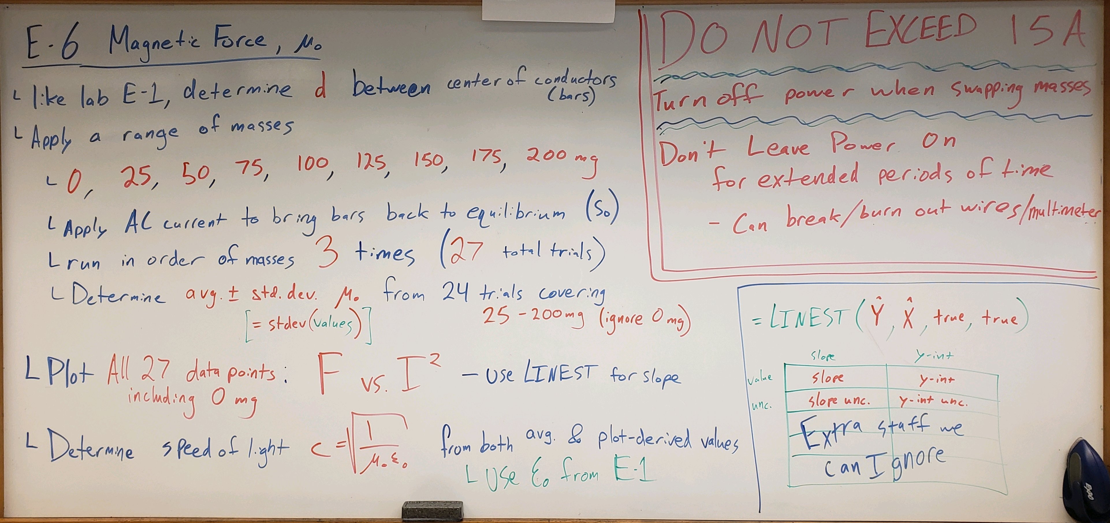
Figure 3:Overview. LINEST() function.
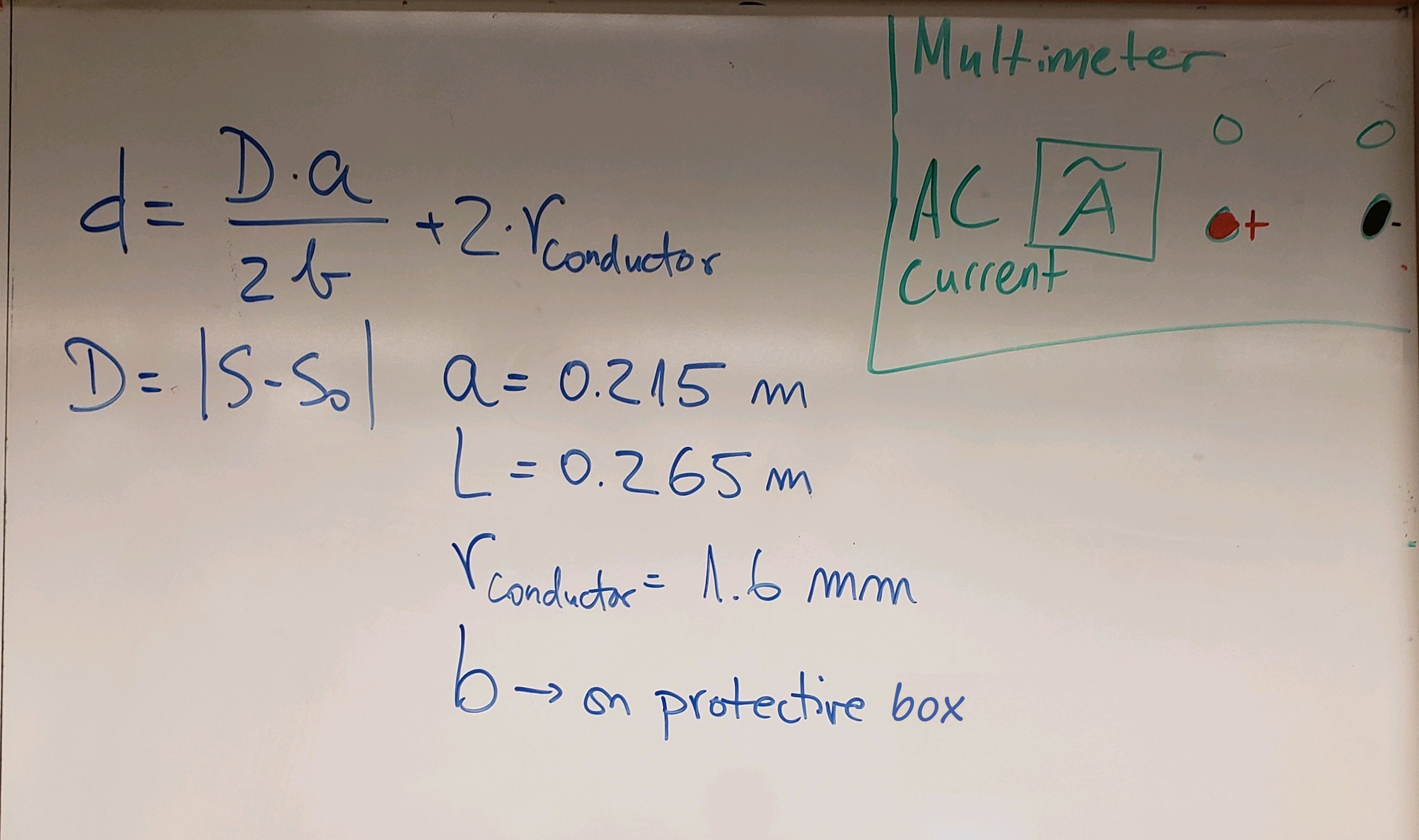
Figure 4:Separation distance equation; multimeter settings.
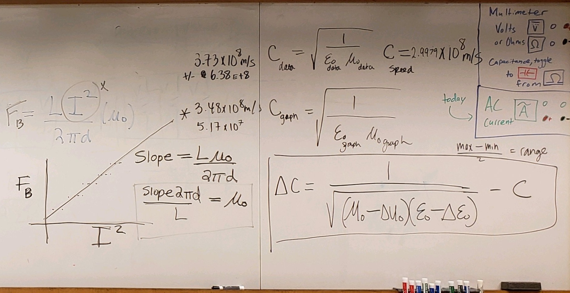
Figure 5:Plot notes; Speed of Light calculations.