1172L-ONLY | Faraday’s Law of Induction
Background
● Background Overview
Today’s experiment will cover two main parts. The first will focus on characterizing the magnetic field near the center of a horseshoe magnet for use later. It will continue by determining average EMF (voltage) and magnetic flux of the induction wand (loops of wire) as it passes through the horseshoe magnet. The second part focuses on characterizing energy lost due to the induced EMF on a closed circuit in addition to frictional effects.
● Magnetic Flux
The magnetic field in a volume of space can be described by vectors, which give the strength of the field (its magnitude) and the field’s direction at each point of the volume. A closed loop (closed, so that the area of the loop is defined) will then have field vectors “punch through” the area bounded by the loop (see example in Figure 1).
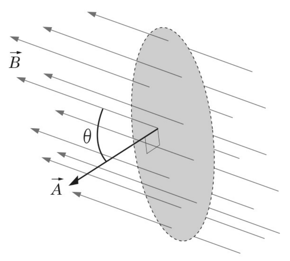
Figure 1:Overview.
One can think of this as the field “flowing” through the area defined by the loop (very similar to water flowing through a cross sectional area of a pipe). This flux can be defined by:
Note that, the right-hand side of the equation holds only if is constant over the area defined by the loop. The flux will be zero if the magnetic field is parallel to the area of the loop and maximum if the field is perpendicular to the area of the loop.
● Faraday’s Law
If a loop of wire (for example a coil) is moving into or out of a magnetic field or if the magnetic field over the area of the loop itself changes (either direction or magnitude), then an electro-magnetic force (EMF, essentially induced voltage) might be induced in the loop due to the fact that the magnetic flux through the loop changes. Faraday’s Law states that the induced electro-motive force [EMF] or voltage in the loop is directly proportional to the rate of change of the flux through the loop. In this experiment, the magnet and coil are arranged so that the magnetic field is perpendicular to the coil loops and:
Here is the number of windings in the coil and the negative sign in front of the expression indicates that the EMF is induced in such a way that it opposes the change in flux through the loop (this direction indication is commonly known as Lenz’s Law).
If we were to then integrate (2), knowing for this lab that the area A of the coil is constant, but the B-field through the area defined by the coil will change, we would find (3).
If we were to average over time, we would find the average EMF (again, with unchanging area for today) is:
If the area is integrated from the beginning of the peak to the point where the voltage is zero and the coil is at the maximum field, then will equal the maximum field. Capstone has an area function  that can be used to measure the integral of the voltage.
If the coil is in a closed circuit with total resistance then a current will flow through the coil according to Ohm’s Law:
The circuit will dissipate energy at a rate of:
Since power is work per time, the energy that is lost in the circuit can be found by calculating the area under the power vs. time graph (i.e. the integral of the Power over time ):
● Energy in a pendulum
The center of mass of a pendulum starting at an initial height , then swinging through its lowest point and finally rising to a height , will experience a change in potential energy of:
If no energy was dissipated, then the change in potential energy would be zero (no potential energy would be lost in this case). If the final height were less, as indicated by the smaller final angle in Figure 2, then the change in energy would give the energy lost during the motion:
Finally the initial and final heights can be related to the angles and the pendulum makes with the vertical direction at these location (see Figure 2):
In this equation indicates the distance from the center of mass to the pivot of the pendulum.
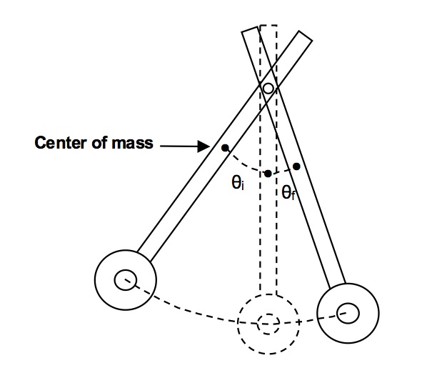
Figure 2:This picture shows the coil wand swinging from an initial angle to a final angle . The final angle is less because of energy lost in the process, which reduces the potential energy by an amount (see (10)).
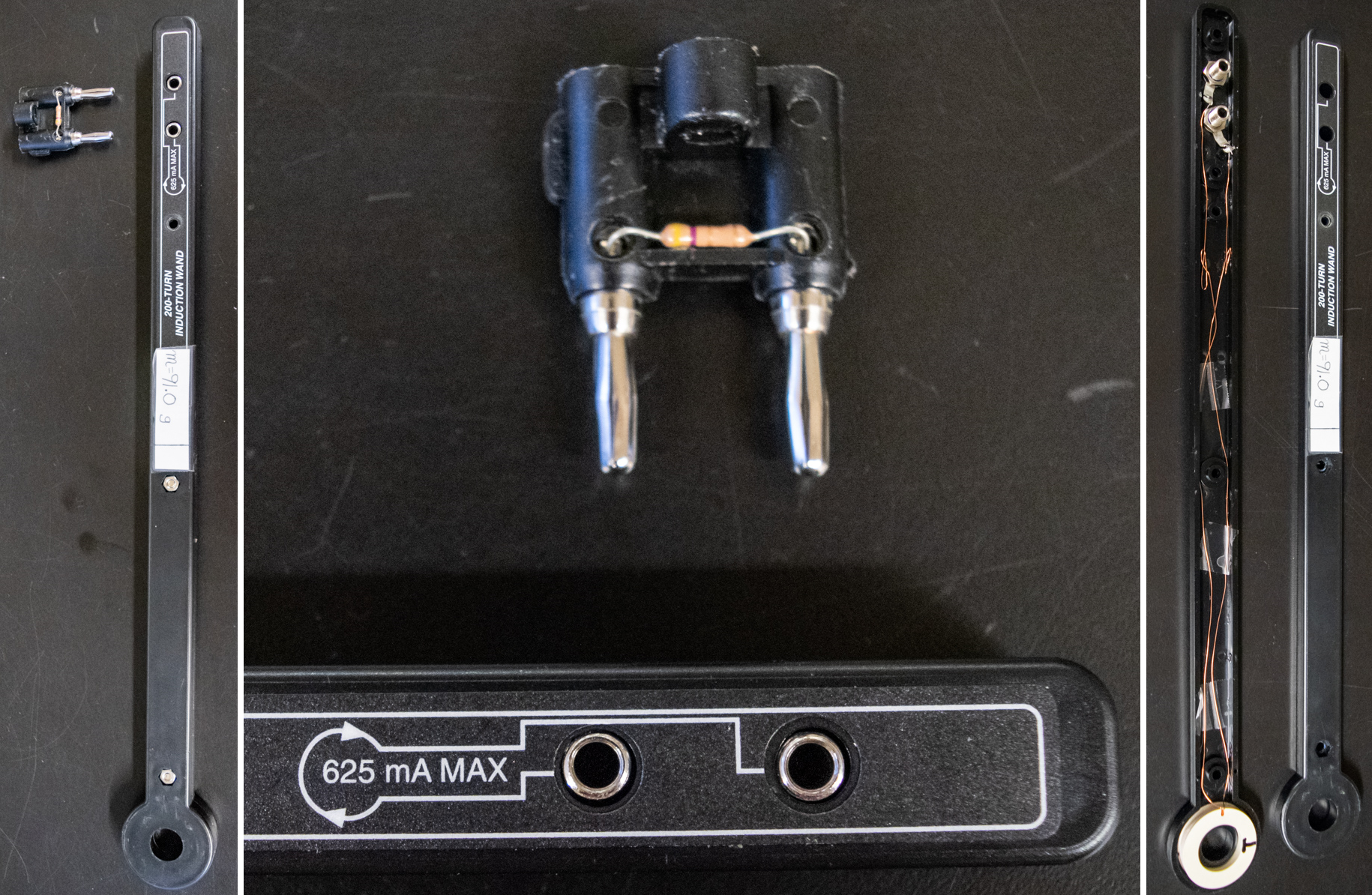
Figure 3:Left) Coil wand with resistor and an example of the center of mass line and mass noted on the wand itself. Center) Resistor and circuit diagram of the wand; resistor plugs in and completes the circuit allowing energy to be dissipated. Right) Internals of the wand; wires lead from the ports to the coil at the bottom of the wand. The area of the loop refers to the area inside the white loop of wire at the bottom.
● Equipment
Table 1:Equipment
| Category | Items |
|---|---|
| Magnetic Source | • Variable gap horseshoe magnet |
| Induction Apparatus | • Induction wand (Figure 3) • Coil parameters: , • Mass and center of mass labeled on wand |
| Electrical Components | • resistor (measure actual value for confirmation) • Can be inserted into wand to complete circuit and measure resistive energy dissipation |
| Mounting Hardware | • Stand, rods, and clamps |
| Voltage Measurement | • Voltage sensor recorded by Capstone • Measures induced voltage in coil • Red/black leads connect to coil wand terminals • Connected to analog input with sample rate |
| Magnetic Field Measurement | • PASPORT 2-Axis Magnetic Field Sensor • Axial: positive into end of probe • Perpendicular: positive upward through probe towards tare-button side • Perpendicular used to measure maximum horseshoe magnet field strength |
| Rotational Measurement | • Rotary Motion Sensor (RMS) connected to Capstone • Measures angular displacement, velocity, acceleration • 3-step pulley attached (see Figure 4) • Coil wand mounted to pulley for rotational measurements • Sample rate , zeroes its position when Capstone starts recording |
Experimental Procedure
● Preview
● Part I: Preliminary Setup
The experiment should be already set up for you as shown in Figure 4. If not, match the figure to include the magnetic pole plates (CAREFUL WITH FINGERS, ASK FOR ASSISTANCE AS NEEDED).
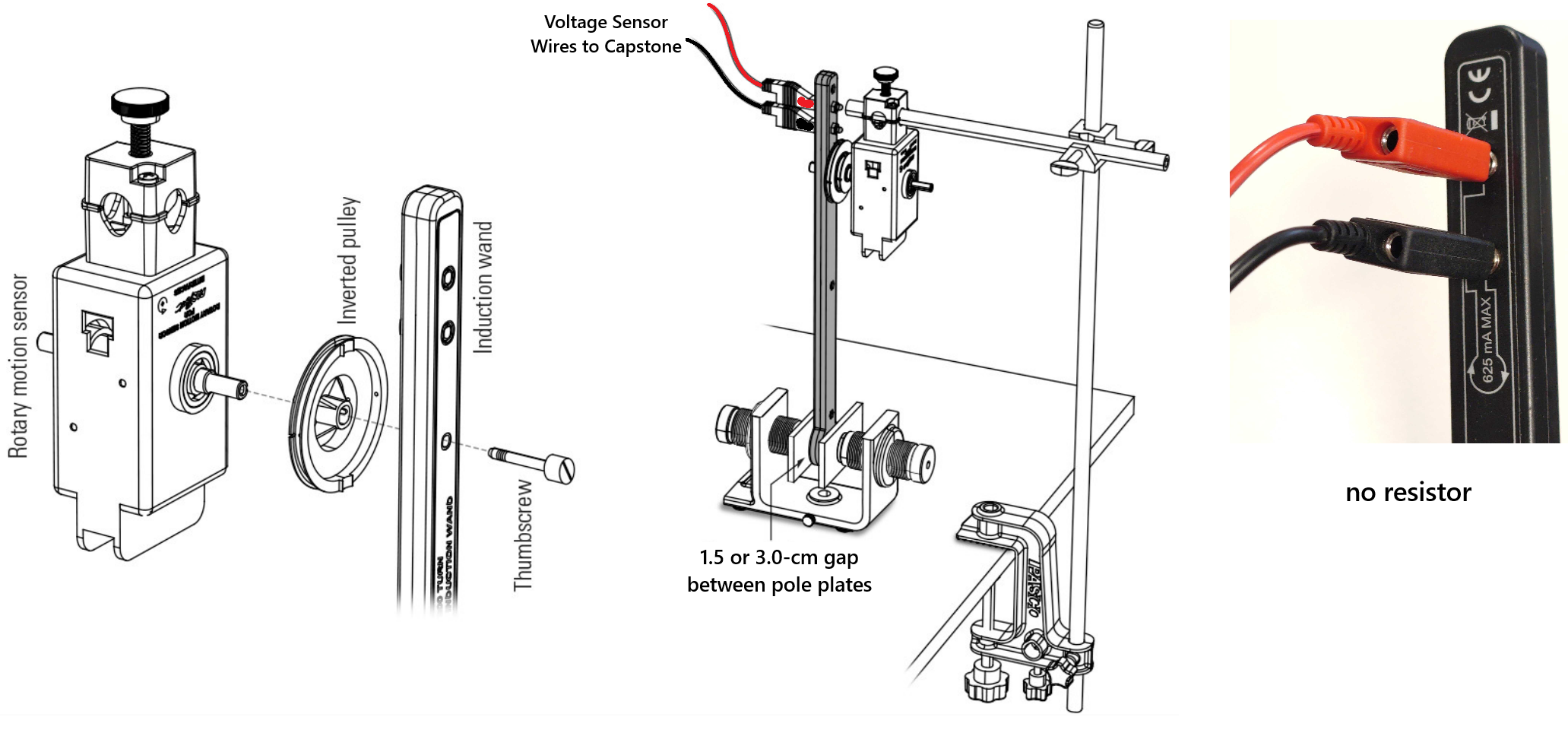
Figure 4:Overall experimental setup consisting of induction wand mounted on the RMS as well as the horseshoe magnet. The cables connecting to the voltage sensor are plugged into the two jacks at the top of the wand.
○ Part I.1: Magnetic Field
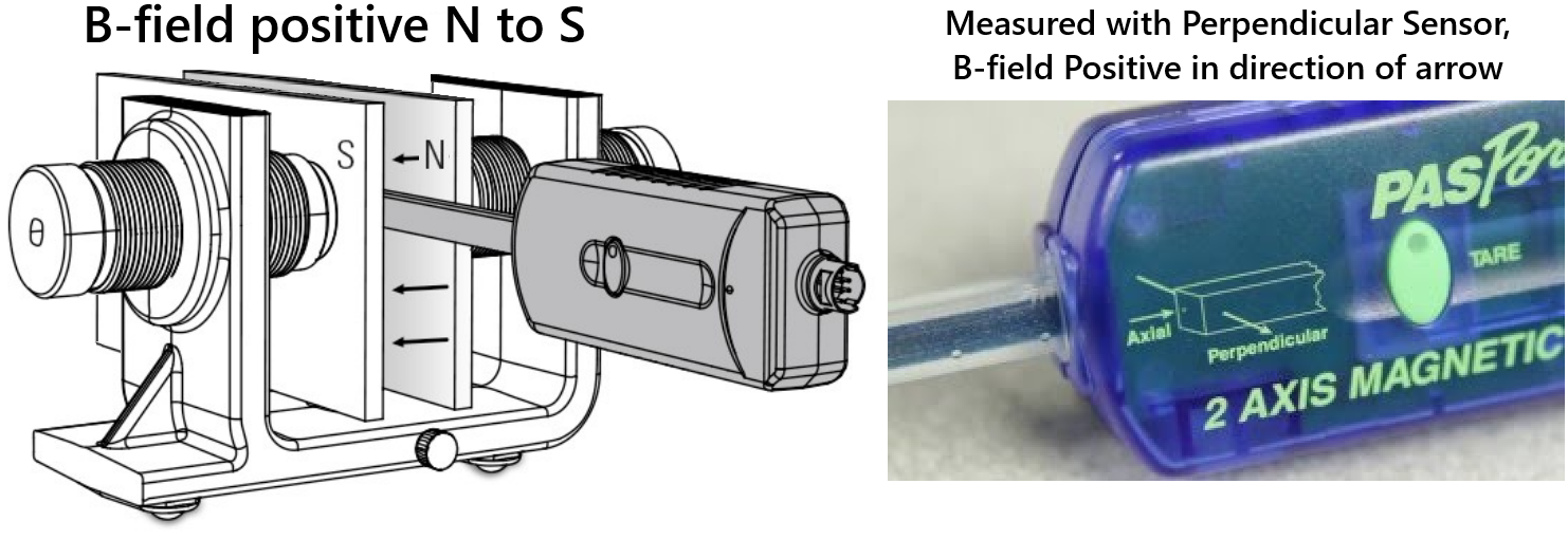
Figure 5:How to measure positive magnetic field strength of horseshoe magnet. Use the perpendicular sensor on the PASPORT 2-Axis Magnetic Field Sensor which measures B-field as positive from North to South or out-of-the-page as illustrated on the sensor casing itself in the right-hand side image.
Set gap between the plates on the magnet to (Case 2 will be ).
Starting in the first tab in the Capstone file, click Record and use the magnetic field sensor to measure the magnetic field strength between the poles of the magnet. First press the Tare button on the 2 Axis Magnetic Field Sensor with it held far from the magnets. Hold the field sensor sideways (same position as in Figure 4) and insert the tip into the gap between the poles of the magnet. When the measured field is positive the label of the magnetic field sensor points towards the South pole of the magnet. The magnetic field direction as measured (positive or negative) is as shown in the diagram on the sensor. The field lines coming out of the side of the sensor with the diagram and tare button on it indicate the magnetic field strength as positive, pointing North to South when external to the magnet.
Hold the Induction Wand pendulum up out of the way. Insert the Magnetic Field Sensor probe between the magnetic pole plates. If the pole plate on the same side as the label on the magnetic field sensor is a south, the Magnetic Field Sensor signal is positive.
Click RECORD. Use the Magnetic Field Sensor to determine which pole plate is north and put a label on it. You will need that for the Lenz’s law part of the experiment. If a compass is available, check to make sure you have labeled your magnet correctly.
Use the Magnetic Field Sensor to probe the field between the plates. Record the maximum field at the center of the plates.
Determine the distance from the horseshoe magnet where the field drops to less than (essentially zero). You will start the coil wand swinging this far from the magnet so that it begins its swing in approximately zero field. Enter your values in the Magnetic Field Data table.
Click STOP.
○ Part I.2: Induced EMF (Voltage)
In this section you will compare the calculated and experimental (EMF or voltage) induced in the wand’s coil.
The coil should be able to move freely through the gap between the magnet poles, with the poles as close together as possible (about between the plates) without restricting the motion of the coil. The center of the coil should be moving right through the middle of the poles. The long axis of the plates is horizontal so the pendulum swings through a more uniform magnetic field.
Switch the Capstone file to the second tab, with Voltage vs. time and angle vs. time plots.
Ensure the Voltage Sensor banana plugs are plugged into the banana jacks on the end of the coil wand. Drape the Voltage Sensor wires over the rods so the wires will not exert a torque on the coil as it swings.
Let the pendulum hang at rest. Press RECORD, and ZERO the voltage sensor by looking in the bottom recording bar, with the voltage sensor selected, click the zero button (zero with two yellow arrows pointing towards each other).
You can now pull the pendulum back. Let the pendulum swing freely and ensure the pendulum can swing 10 oscillations over about 10 seconds. If it’s longer, you may have extra friction from the wand hitting/scraping against the magnet or wires. No data is needed for this step, just double check your setup. Once you’re sure the pendulum can freely swing, move on to the next step.
WITH THE PENDULUM AT REST, click RECORD and pull the coil wand out a bit further than the zero-B-field position you measured in step 2 above (). Release the wand and let it swing through the magnet out and back once (see Figure 6). Then click STOP. The graph should show at least four pulses similar to Figure 7.
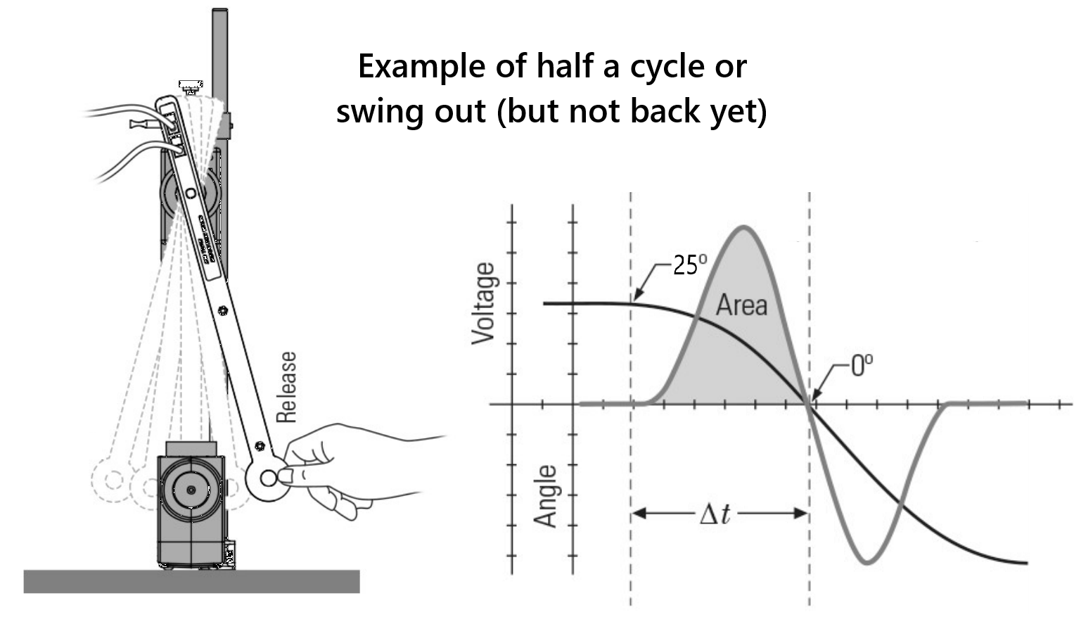
Figure 6:Example of releasing the wand and example of just half a cycle the start/stop times and area under the curve for just the first peak.
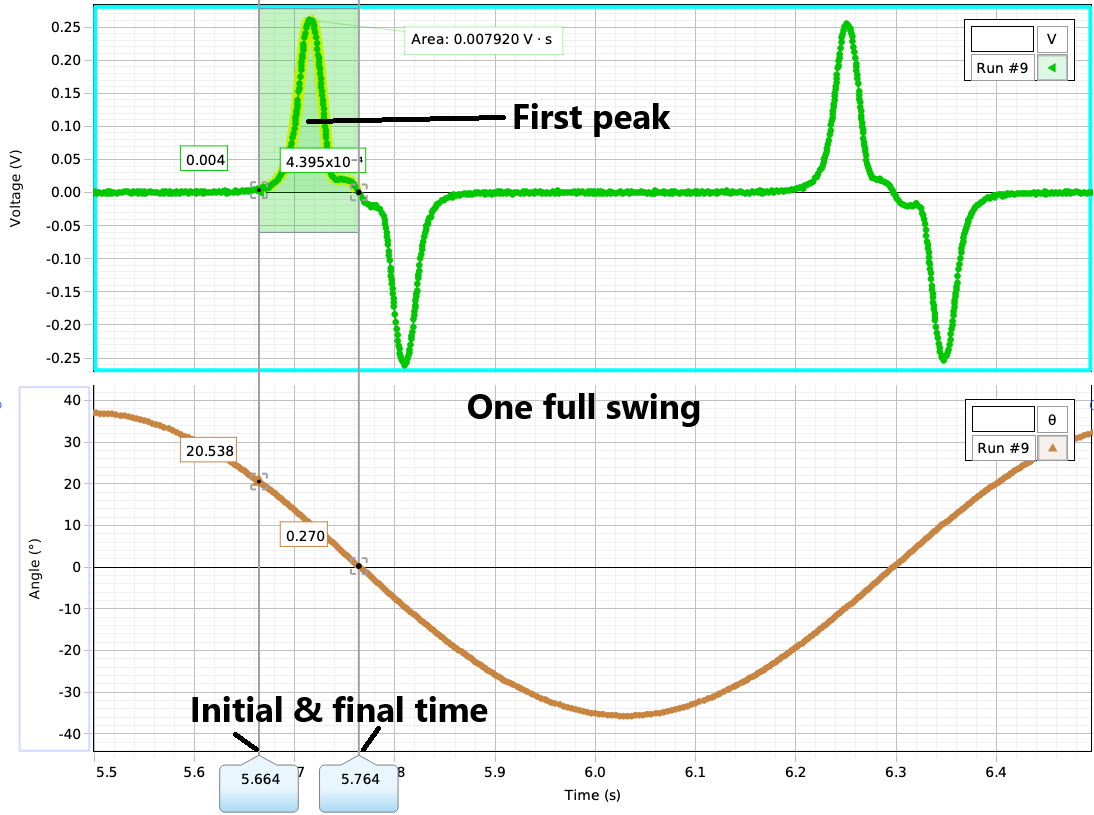
Figure 7:Example of plots for this part.
Press the “Stop” button on Capstone.
Enlarge the portion of the voltage vs. time graph where the coil passed through the magnet.
Enable and use the Multi-coordinates tool
 to determine the difference in time from the beginning to the end of the first peak.
Record initial and final times (see Figure 6).
Find the average EMF by highlighting the first peak from when voltage lifts off from zero and returns to zero:
Find the experimental area under the curve of the voltage versus time graph for the first peak using the area tool
.Calculate your experimental value of the average EMF using your plot-derived values and the left-hand side of (4). (The integral is the area under the curve)
Calculate the expected value of the average EMF using the right-hand side of (4).
Compare your experimental and expected values with a percent difference (reminder in Difference Between Experimental and Expected Values).
Use for the number of turns of the coil and for its area.
Find change in Magnetic Flux through a single loop
Determine your experimental change in Magnetic flux for a single loop using your average EMF value and (4) (think back to (1) on what magnetic flux is).
Calculate the expected change in magnetic flux for a single loop calling back to (1).
Compare your experimental and expected values with a percent difference (reminder in Difference Between Experimental and Expected Values).
PLOT 1 of 2 --- for just the first case (): take a photo/screenshot of Capstone’s Voltage vs. Time and related Angle vs. Time for one full swing (out and back, example in Figure 7).
Increase the magnet gap to and repeat previous steps, still releasing the pendulum from the same position you used before.
○ Part I.3: Lenz’s Law
Think about this section as you will need to cover it in your post-lab submission.
Look at the circuit diagram showing the coil orientation printed on the Induction Wand (also shown in Figure 3). Note that we have connected the red plug from the Voltage Sensor to the upper port and the black plug to the lower port. If coil current flows in the direction shown by the arrows (clockwise), then the upper port becomes positive due to excess positive charge there, and the lower port becomes negative due to decrease in positive charge. Since the red lead from the Voltage Sensor is attached to the upper port, the Voltage Sensor would read a positive voltage. Caution: although current flow in an external circuit is from positive to negative, current flow inside a battery or power supply must be from negative to positive.
Lenz’s Law states that the current induced in a coil by a changing magnetic field through the coil will flow in a direction to oppose the change which produced it. In particular, the field produced by the induced current will be in a direction to try and prevent the field through the coil from changing.
The magnetic field points from the north pole to the south pole. As the coil enters the magnet, the magnetic flux increases in that direction. Lenz’s Law says that the induced voltage opposes the change in flux.
● Part II: Energy Conservation Preliminary Setup
Measure resistance of both the induction wand itself and the resistor itself.
With the coil outside of the magnetic field, use an ohmmeter to:
Measure the resistance of the coil in the induction wand. Why must the coil be out of the field of the horseshoe magnet when measuring resistance?
Verify the resistance of the resistor.
In Capstone, go to the next page. On the left side, click on the calculator. Update the resistance values in the calculator to be accurate to your setup and click accept. Finally click the calculator to close it. Before you start any additional trials, click the calculator to make sure the resistor values are correct and have not reverted to the default values.
Change the setup to match Figure 8.
Remove the magnet pole plates. (ASK FOR ASSISTANCE AS NEEDED) Move the magnets as close to each other as possible, making sure that you leave enough space for the coil to move through the gap.
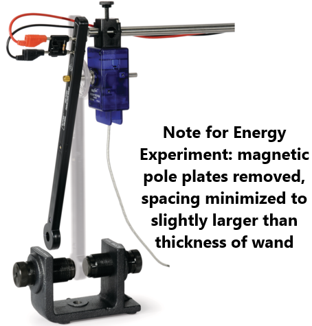
Figure 8:This picture shows the overall setup for the current part. Note: magnetic pole plates are removed and magnet spacing shrunk. Resistive load attached to the coil wand. The cables leading to the voltage sensor are plugged into the resistor.
Connect the voltage sensor wires with the resistor into the coil wand.
Make sure for the first part (friction only), only half of the resistor is plugged so current does not flow, but the weight distribution stays consistent (see Figure 9). Check that the alignment generally matches the alignment you will have later when the resistor is plugged in (○ Part II.1.B: Energy Lost due to Only Resistor).
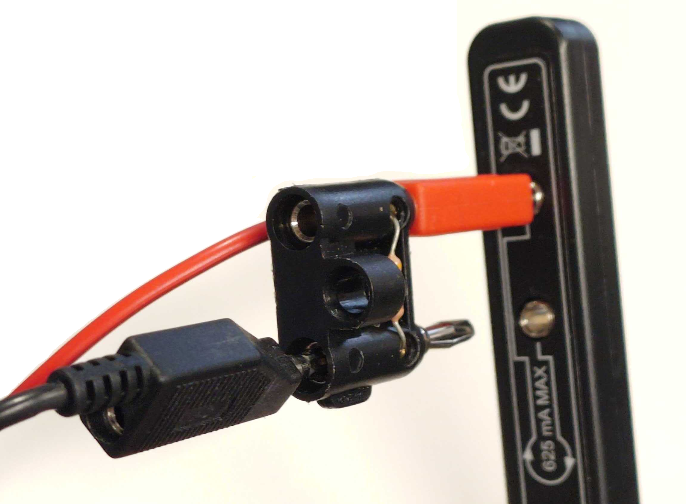
Figure 9:This picture shows the resistor half plugged-in.
Measure the distance of the center of mass of the wand (marked on the white piece of paper taped to the wand) from the pivot (the screw). Note the result in the data table. (see Figure 3)
Note the mass of the wand (also noted on the wand) in your data table.
○ Part II.1.A: Energy Lost due to Only Friction
First determine the amount of energy lost to friction by letting the pendulum swing through the magnet with the resistor disconnected. Reminder, this is done by having the resistor plugged into the wand with only one of the banana plugs connected (see Figure 3). This makes sure that no current flows through the wand (and the resistor) while leaving the center of mass of the wand relatively unchanged.
Press the “Record” button on Capstone with the coil at rest between the magnet poles. The rotary sensor zeros itself out whenever you start recording, we want to make sure is when the wand is at rest inside the magnet.
Rotate the wand to an initial angle of and let it go.
Press the “Stop” button after the wand has reached the other side.
Zoom in to the portion of the angle vs. time graph where the coil passed through the magnet. Select the peak and get the maximum (initial) and then the minimum (final) angle of the motion to find the initial angle () and the angle to which the pendulum rises after it has passed once through the magnet (). (see Figure 10-bottom)
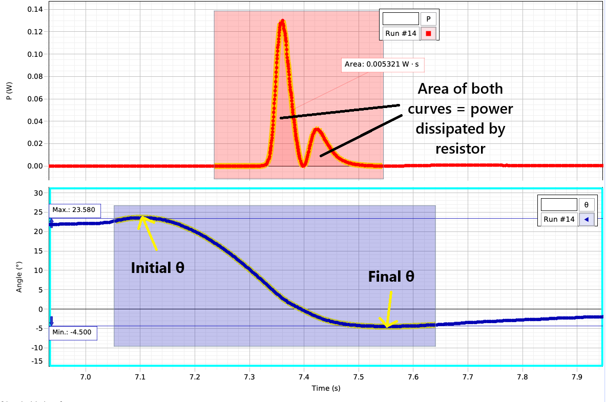
Figure 10:Example of plots for this part.
Calculate the energy lost to friction using (10).
○ Part II.1.B: Energy Lost due to Only Resistor
Now connect the resistor by plugging in both plugs in series with the wand (Figure 11).
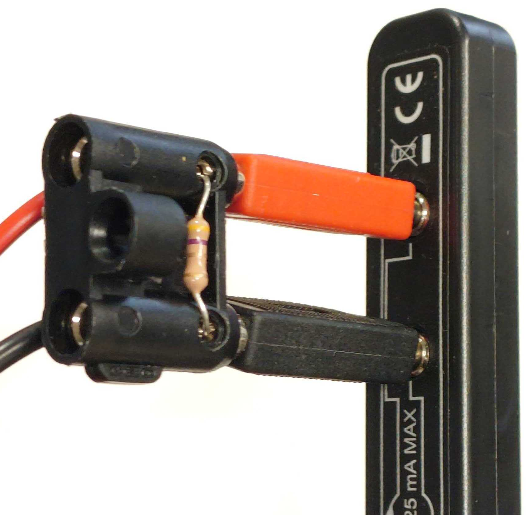
Figure 11:The resistor fully plugged-in.
Press the “Record” button on Capstone with the coil at rest between the magnet poles.
Rotate the wand to an initial angle of and let it go.
Press the “Stop” button after the wand has reached the other side.
Detemine energy dissipated by the resistor.
Highlight both peaks on the power vs. time plot and find the area under the curve (area tool
).Right-click the displayed value to set the numeric format and increase sig. figs. Record this area as it equals the the energy dissipated by the resistor as presented in (7).
○ Part II.2: Energy Lost Overall
Using the same data run as Part II.1.B, measure the initial angle () and the angle to which the pendulum rises after it has passed once through the magnet (), but now that the resistor was fully plugged in.
PLOT 2 of 2 --- for just when the resistor was plugged in: take a photo/screenshot of Capstone’s Power vs. Time and related Angle vs. Time for one-half swing (out but not back, example in Figure 10).
Calculate the total energy lost using (10).
Compare this total energy lost value (Part II.2) to the sum of the energy lost due to friction (Part II.1.A) and the energy dissipated by the resistor (Part II.1.B).
Calculate the percent difference between the two.
● Summary & Cleanup
Create a summary table of your data (e.g. relevant final result values and percent differences from Part I and Part II).
When you are finished, reset your experimental setup before leaving.
Post-Lab Submission --- Interpretation of Results
● Finalized Spreadsheets
Make sure to submit your finalized data table (Excel sheet).
Please include concise summary table.
Please include plots (from Capstone):
vs time and related Angle vs. Time (Part I) for one full cycle or swing out and back
vs time and related Angle vs. Time (Part II) for one-half cycle or swing out (but not back) when resistor is in circuit
● Post-lab Writeup
In a paragraph, summarize your error analysis. Be both qualitative and quantitative.
What is the precision of your equipment?
What are possible sources of systematic (i.e. affecting accuracy) and random (i.e. affecting precision) errors?
What are your measurement uncertainties, and, based on these uncertainties, which impact your final results the most?
In a paragraph, summarize the results you have determined for all cases. Consider:
What was the point of today’s lab; what did we aim to discover?
PART I
Do your experimental results for average EMF and change in flux from part 1 agree with the expected values? By how much?
What was the induced voltage of the coil of wire swinging into the magnetic field dependent on?
Looking at your plot from Capstone of Voltage vs. Time, there should be four spikes in voltage during one whole cycle forward and back.
Why are the first and second peaks opposite signs (positive vs. negative, look back on the wand’s circuit diagram and think about how current would flow), and how does that relate to Lenz’s Law?
Why is the voltage zero as the coil passes through the center of the magnet?
Does it matter which direction the coil is moving or which direction the magnetic field is pointing?
PART II
Do your values for total energy loss (with resistor) agree with the sum of the energy dissipated by the closed circuit (with resistor) plus friction of the rotary sensor (without resistor)?
Why would you expect them to agree? Why physically was energy lost?
Why, for the Power dissipated vs. Time plot were there two peaks, but now of the same sign (i.e. both positive)?
Why, if you used a larger resistor, for example a resistor in place of the resistor, should the damping of the pendulum would be reduced?
The Whiteboard
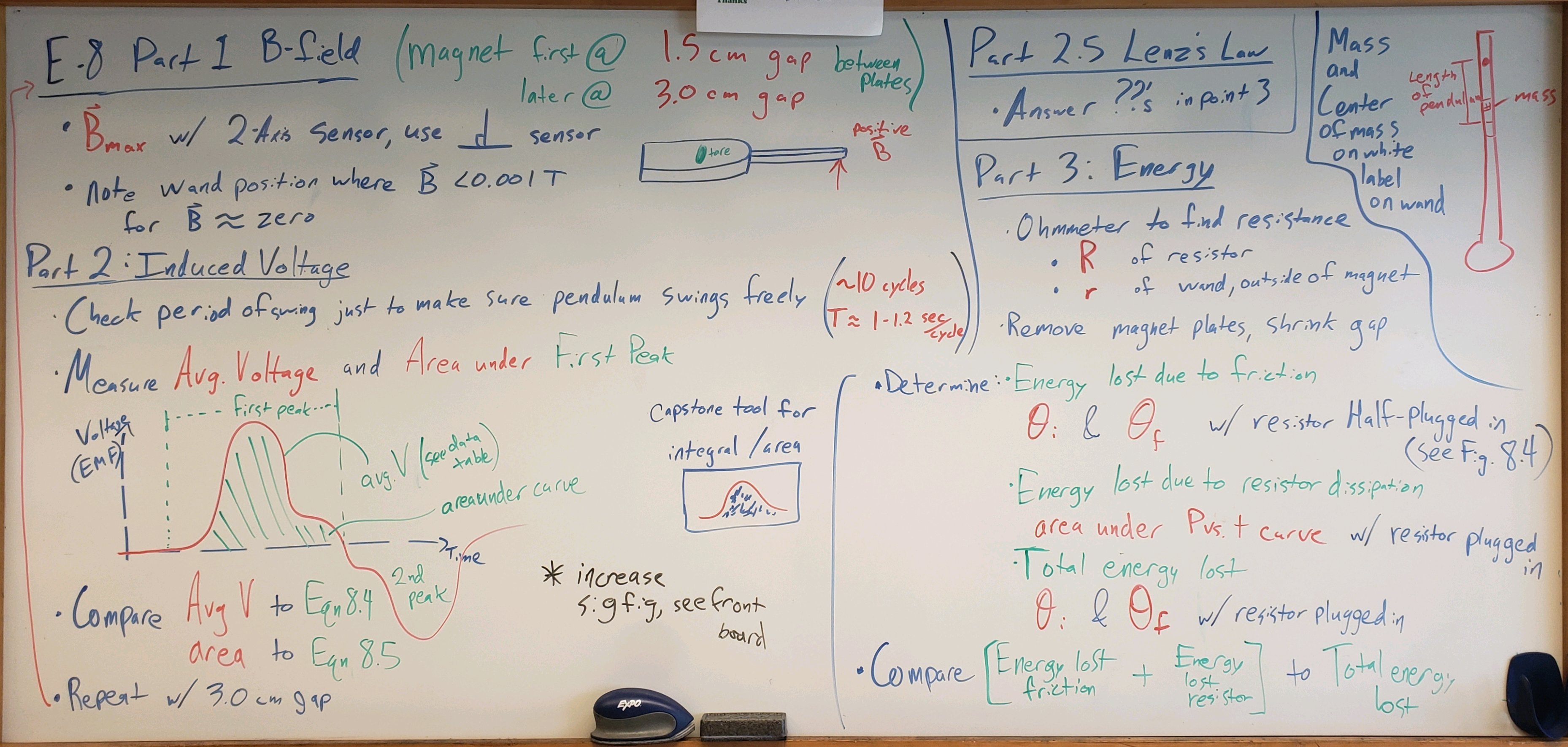
Figure 12:Old overview, majority still the same, but different induced voltage values to find.
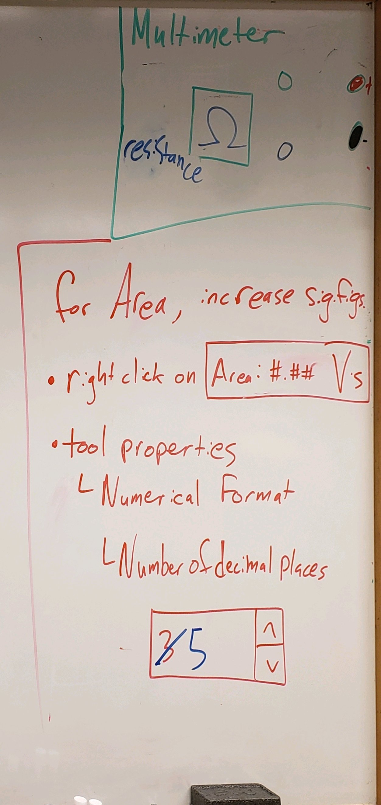
Figure 13:Multimeter settings, changing significant figures in Capstone (must be done every new data run).
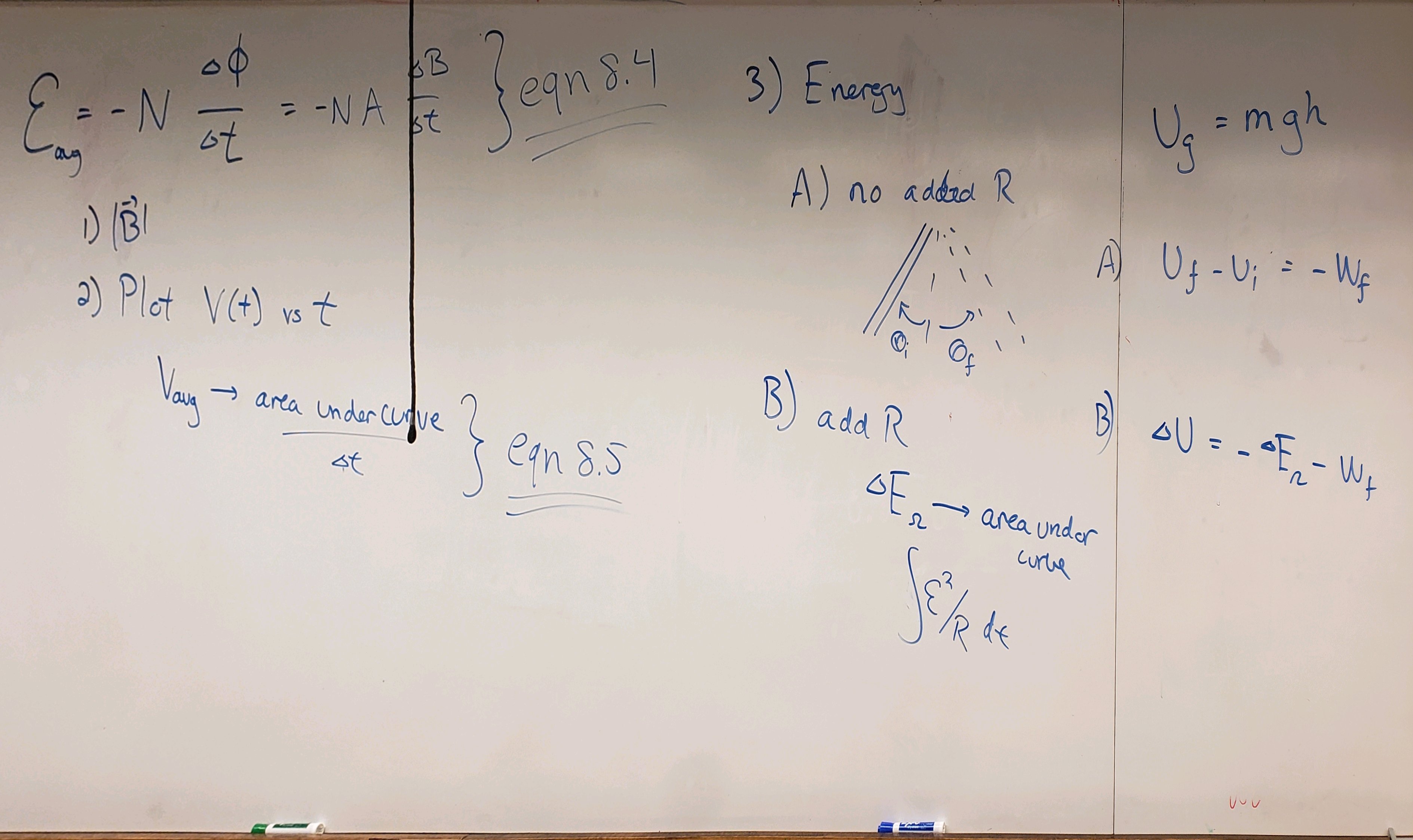
Figure 14:Short notes on the three parts of the lab.