Electric Force & the Determination of ε₀
Background
● Background Overview
The electric constant, (pronounced “epsilon nought” or “epsilon zero”), is a fundamental constant of nature. Also known as vacuum permittivity, permittivity of free space, or dielectric permittivity of the vacuum, it is a measure of how dense of an electric field is “permitted” to form in response electric charges. As such, it is also the proportionality constant that relates the electric force between two charges. The constant is also related to the constant in Coulomb’s Law which describes the electrostatic force between charges:
where is the charge in Coulombs, is the separation distance between charges in meters, and
The subscript zero refers to the baseline value of the permittivity of free space.
● Electric Force Between the Plates of a Parallel-Plate Capacitor
If we apply Coulomb’s law to the special case of two large, closely-spaced, parallel plates, we can derive an expression for the electric force between the two plates. This electric force is due to the uniform electric field generated between this configuration known as the parallel-plate capacitor as seen in Figure 1.
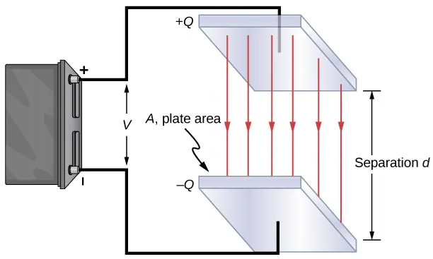
Figure 1:Example of a parallel-plate capacitor. Plates of area are seaparated apart with charge built up on each plate based on the applied voltage which creates a uniform electric field.
A parallel-plate capacitor with idential plates of the same surface area A separated by a distance d, each plate has the same surface area A.
Consider such a parallel-plate capacitor with plate area , separation , and an applied potential difference . When a voltage is applied, equal and opposite charges accumulate on the plates, producing a surface charge density
○ Electric Field of the Plates
A single (ideally) infinite sheet of charge with surface charge density produces a uniform electric field one either side of that sheet with a magnitude
In a parallel-plate capacitor, the two plates carry equal and opposite surface charge densities . The electric fields due to each plate add between the plates and cancel outside the capacitor, resulting in a uniform electric field between the plates:
Because the field is uniform, the potential difference between the plates is related to the field by
where to increase the electric field strength, you can either increase the voltage or decrease the separation distance between the plates.
○ Force on a Plate
A key point is that a charged plate does not exert a force on itself. The force on one plate arises solely from the electric field produced by the other plate.
The electric field at one plate due to the opposite plate alone is therefore
The force on a plate carrying total charge (i.e. the electric force that the charges on the one plate feel due to the other plate’s electric field) is
Substituting gives
○ Force in Terms of Voltage
Using the relation between surface charge density and electric field,
the charge on a plate becomes
Substituting this expression for into the force equation yields
○ Final Result
The following expression gives the magnitude of the attractive electric force between the oppositely-charge plates of an ideal parallel-plate capacitor.
where is the area of the plates, the separation distance, and the potential difference in volts between the plates of the capacitor.
(13) is valid only under the conditions stated of large, closely spaced plates to provide a uniform electric field and charge density so we can effectively ignore fringe fields. The physical implications of these geometric assumptions is that the electric field is totally confined to the space between the plates and is constant in value throughout the space. You will see in Lab E-2 that the electric field always ‘bulges’ or fringes out at the edge. For (13), the fringe field is ignored. Rewriting the expression for , we obtain
By measuring electric force, voltage, and geometry of the apparatus, can be determined.
● Equipment List
Depicted across Figure 2 -- Figure 5. All equipment as listed can be seen first in Figure 2.
Telescope with crosshair & centimeter-scale ruler (a.k.a. scale) on vertical pole
High voltage DC power supply, 0 -- 500 V
Fluke multimeter -- set to read DC voltage (in parallel with parallel-plate capacitor)
Small masses of 10, 20, 20, 50, 500 mg with plastic tweezers
Parallel-plate capacitor apparatus:
Bottom plate held in static position on lower plate adjustment towers
Balanced plate/beam on thin, conductive, knife edges with:
Top plate with a “” for where to place applied masses
Can swing up or down when changing amount of applied mass or voltage
Set up to be parallel (i.e. equilibrium) to bottom plate when holding
Mirror to view the scale (ruler) via telescope to determine angle of plates and subsequent separation distance between plates
Beam lift knobs to reset top plate position after accidental bumps
High impedance () resistor to limit current (contained in long gray box, shouldn’t need to touch)
Leveling screws to level whole apparatus to the table
Metal connections to the power supply
5x Banana plug wires (12 AWG: 2x 3’, 1x 1’; 18 AWG: 2x 2’), connecting power supply to voltmeter & parallel-plate apparatus
Protective box with the mirror-to-scale distance written on it
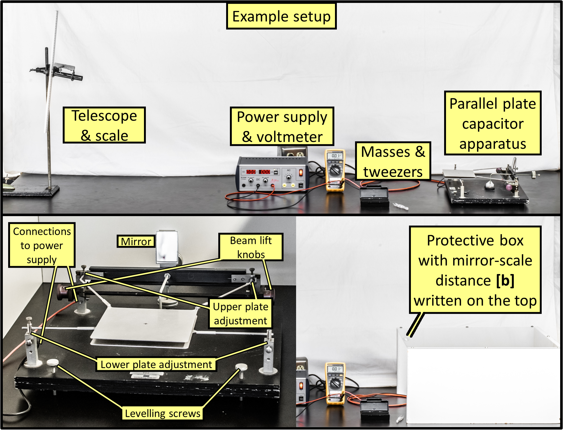
Figure 2:Top) Example of the entire setup (note: actual setups will have telescope/scale on separate table further away). Bottom) Front view of capacitor apparatus; protective box.
● Adjustment of apparatus (check with Instructor if needed)
The apparatus has been carefully adjusted before your lab and should not require further significant adjustments. This section describes how the apparatus was prepared. If something seems to need adjusting, see the lab instructor.
The beam lift (knob location noted in Figure 2 bottom-left) provides a definite location for the beam and thus guarantees continued alignment of the parallel plates. Use the beam lift each time you change weights or relocate the counter weight.
Both plates can be adjusted vertically and horizontally in order to make it possible for the plates to be parallel. The counterweight behind the mirror can be used to establish the equilibrium separation of the plates. The plates should have already been adjusted parallel with the counterweight set so the plates are essentially parallel when a mass is placed on the movable plate. If the plates are NOT parallel with the mass in place, seek the instructor’s help.
The apparatus can be leveled with the leveling screws so that it sits flat on the table.
Mirror-to-scale distance was measured from rear of mirror (reflective surface) to ~center of and on the scale (ruler).
Demo Video: Setup & Procedure
Demonstration video. Reviews overall setup and procedure. *No audio*
If embedding is broken, follow: https://
Experimental Procedure
● Preview
● Preliminary Setup
All given lengths you will use are represented in Figure 3.
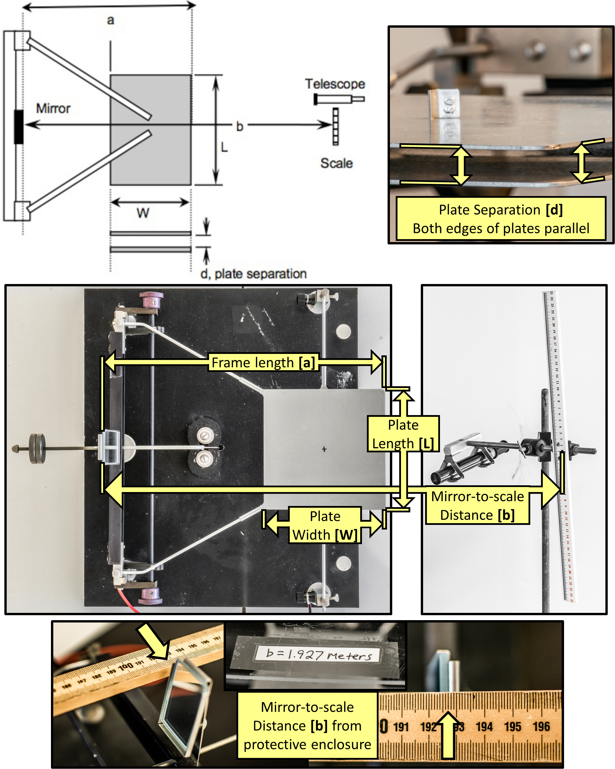
Figure 3:Parallel Plate Capacitor Apparatus. Top-left) Schematic showing given dimensions and determined plate separation . Top-right) Determined plate separation when parallel (i.e. at equilibrium with no applied voltage). Middle) Example apparatus with given dimensions. Bottom) Example of mirror-to-scale distance.
Prepare a common data table including given values. Reminder -- keep variable names and units in the row and column titles, and numbers in their own Excel cells to be able to reference in your equations. Include, but not limited to:
: Accepted value of accel. due to garvity for Fairfield University
: Accepted value of electric constant
: Length of the frame from pivot to end of plate (see Figure 3)
: Mirror-to-scale distance, has already been measured and is posted on the top of the protective enclosure (Figure 3 bottom)
: Plate area (Figure 3)
: Equilibrium mass (plates are parallel when this amount of mass applied).
: Equilibrium force
: Scale reading at equilibrium (m)
: Scale reading when plates are in contact (m)
: Separation distance between the plates when the top plate is parallel to the bottom plate when equilibrium mass () is placed on the top plate (see examples in Figure 3 top-right and Figure 5 middle)
Note the center marking “+” on the top of the movable plate where masses must be placed using the tweezers (see Figure 4).
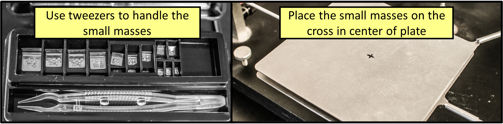
Figure 4:Example of masses to use (milligrams). Placement location marked by the +.
Investigate the use of the telescope and scale so that the rotation of the balanced frame can be measured in terms of scale divisions (see Figure 5). Numbers are in cm, small lines in mm.
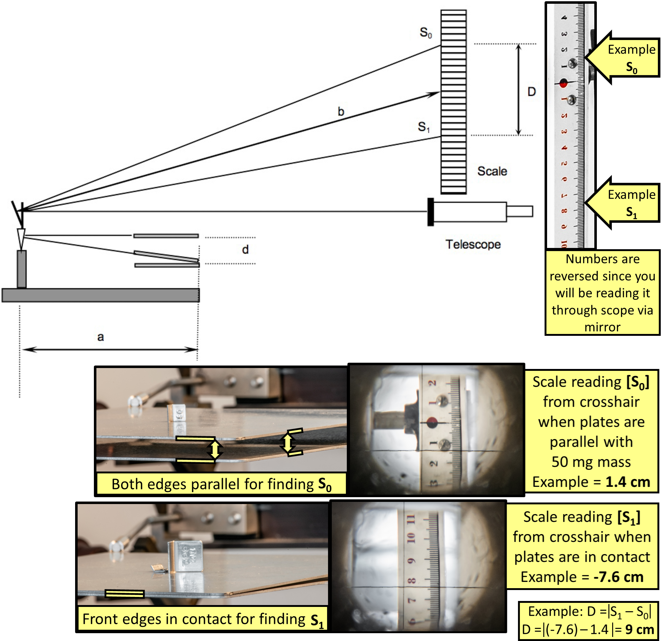
Figure 5:Top-left) Schematic of the Measuring Apparatus. Top-right) Example of and on the scale. Bottom) Example of the plates and cross-hairs through the telescope for finding , , and scale difference . Note for the and readings, the scale numbers are black and red, respectively; this indicating we crossed the zero line and changed signs.
Review the Demo Video: Setup & Procedure. Determine separation distance of the plates when they are essentially parallel with applied. To do so, perform a geometrical analysis of similar triangles that describes the vertical displacement of the plate as given by (15). is the change in scale reading between when the equilibrium mass is on the plate and when the plates are in contact (example shown in Figure 5) and and as described earlier (further described in Figure 3). The factor of 2 results from the fact that the optical path reflected off of the mirror to the scale rotates through an angle twice that of the beam holding the movable plate. Determine from two scale readings (reminders: absolute value there is to represent the total distance between and . If your crosshair crosses 0, make sure to consider the negative). Perform the following:
The first scale reading, , is made when the separation of the plates is such that the plates are essentially parallel. This should happen when an applied mass of is centered on the movable plate. If not, call over an instructor.
The second scale reading, , is made when the top plate contacts the bottom plate (Figure 5). Place a sufficient mass (e.g. ) on the movable plate to make it contact the lower, stationary plate
⚠️ POWER MUST BE OFF FOR THIS STEP ⚠️
You will periodically verify that and are not changed throughout the experiment.
Record , , and in your common data table.
Also include the equilibrium mass , the equilibrium force , distance , and distance found on your apparatus cover.
Calculate the plate spacing using (15).
We can now determine an experimental value of from the values in the common data table and the experimental voltage from each trial. You will perform at least three trials for each of the six different applied masses on the movable plate (18 total trials). Set up an experimental data table to record your measurements and calculate the experimental value of . Include enough rows for trials and columns for:
Trial number
Lab member’s initials (person looking through telescope)
: Applied mass
: Applied gravitational force
: Applied electric force (to be calculated later)
: Minimum voltage required to return to the equilibrium position
: Maximum voltage required to return to the equilibrium position
: Voltage required to return to the equilibrium position
: Estimated voltage uncertainty (to be assumed as majority source of uncertainty for today)
: Experimental value of the electric constant
: Maximized experimental value of the electric constant based on
: Uncertainty in experimental value of the electric constant
: Magntitude of difference between experimental and accepted values of
● Experimental Data Collection
Repeat the following steps for each trial with applied masses in order (to catch any procedural issues early):
The order of the trials for applied masses will be
Round 1:
WITH POWER OFF 🟥 --- 50 mg, ensure has not changed
WITH POWER ON 🟢 --- 40, 30, 20, 10, 0 mg
Round 2:
pause, change group member on telescope
WITH POWER OFF 🟥 --- 50 mg, ensure has not changed, re-run Step 4 if needed
WITH POWER ON 🟢 --- 40, 30, 20, 10, 0 mg
Round 3:
pause, change group member on telescope
WITH POWER OFF 🟥 --- 50 mg, ensure has not changed, re-run Step 4 if needed
WITH POWER ON 🟢 --- 40, 30, 20, 10, 0 mg
Replace the equilibrium mass in the center of the top plate with the current trial’s mass . The top plate will swing upwards. In following steps, you will apply an electric force to make up for the removed gravitational force. Record the current mass value and calculate (reminder, use SI units; these masses are in units of milligrams).
Determine applied voltage (read from multimeter) required to return to equilibrium by finding a voltage range. Turn on 🟢 the power supply and slowly increase the voltage until the plates return to parallel (i.e. crosshair in telescope back to , as it was with 50 mg on the top plate). Determine this by having an observer watching the scale reading with the telescope during this process. The telescope observer should be calling out instructions to the power supply operator to slowly approach the value.
When the value is approximately reached, call out to the power supply operator.
Power supply operator shall decrease the voltage until the telescope observer is no longer confident the crosshair is at the position, at which point the telescope observer shall call for a minimum voltage reading from the multimeter (not the power supply) and record the voltage .
Power supply operator shall then increase the voltage until the telescope observer is no longer confident the crosshair is at the position, at which point the telescope observer shall call for a maximum voltage reading from the multimeter and record the voltage .
Calculate applied voltage as the average of the min and max voltages,
Calculate applied voltage uncertainty as half the difference between max and min voltage,
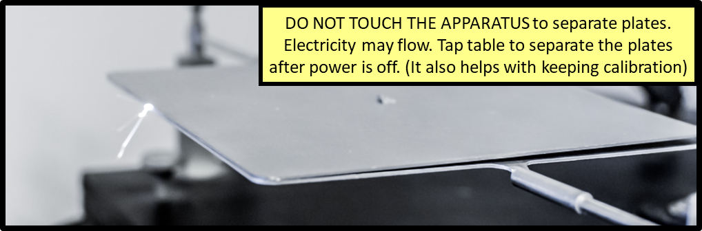
Figure 6:Safety: regarding electricity and the plates touching.
Reduce the voltage to zero and turn off 🟥 the power supply.
For current trial, calculate:
the applied electric force --- the difference between the equilibrium force and the applied gravitational force (see (16)).
experimental electric constant using (14). For trials, this can be ignored as there should be no electric force used.
maximized electric constant assuming uncertainty in voltage is majority source of uncertainty using the form of (17).
Uncertainty in experimental value of the electric constant as
: Magntitude of difference between experimental and accepted values of
Repeat Steps 6 through 10 for the listed mass trials until you’ve completed the listed number of rounds. On the equilibrium trials, check that and have not changed during your experiment.
Check if all the values are reasonably consistent. Retake any data that are clearly erroneous and recalculate.
● Data Analysis
Calculate your average values from everyone’s trials (ignoring the trials):
Average experimental value
Average experimental uncertainty
, the average difference between experimental and accepted
Graphical Analysis: The graphical display of data permits the comparison of all the values and associated errors at once. Points that depart markedly from the general trend of the data are quickly detected. We expect from theory (13) that electric force and voltage are related like:
Using all of your data points from all rounds and trials, including those at equilibrium () that you should have ignored earlier when you calculated for each individual trial and the overall average:
SCATTER PLOT vs. (i.e. as ordinate () and as abscissa ()). Fit a trend line through the all these points, display the trendline equation on the chart, and confirm the slope of the line matches what you found with the
LINEST()function (for review, see Plotting in Excel). From (13), the value of is given by
A slope-derived can now be determined by rearranging (19) and using this experimentally determined value . Thus
Calculate
Similar to earlier, calculate by maximizing the slope by the slope uncertainty (output from the
LINEST()function), and subsequently taking the difference:Also calculate the difference between the slope-derived and accepted electric constant.
SCATTER PLOT vs. . Fit a quadratic trend line, and display the equation.
Create a summary table of your data (e.g. average and slope-derived values with their uncertainties, difference between experimental and accepted value).
When you are finished, reset your experimental setup before leaving.
Post-Lab Submission --- Interpretation of Results
● Finalized Spreadsheets
Make sure to submit your finalized data table (Excel sheet).
Please include relevant plot(s) including:
vs. with all data points across all trials, including those at equilibrium ().
vs. with all data points across all trials, including those at equilibrium ().
● Post-lab Writeup
In a paragraph, summarize your error analysis. Be both qualitative and quantitative.
What is the precision of your equipment?
What are possible sources of systematic (i.e. affecting accuracy) and random (i.e. affecting precision) errors?
What are your measurement uncertainties, and where do they come from?
How do your final results for change based on your uncertainties (e.g. maximizing/minimizing voltage values)? Make sure to have completed error propagation calculations (described in the procedure) in your spreadsheet.
In a paragraph, summarize the results you have determined, including both analysis methods. Consider:
What was the point of today’s lab; what did we aim to discover?
Do your experimental results (average and slope-derived experimental values with their uncertainties) agree with the accepted value for ?
What is the physical relationship between and ?
What physically causes the top (movable) plate to feel an electric force?
Explain physically why you would expect the linear fit to go through the origin of the vs. plot?
The Whiteboard
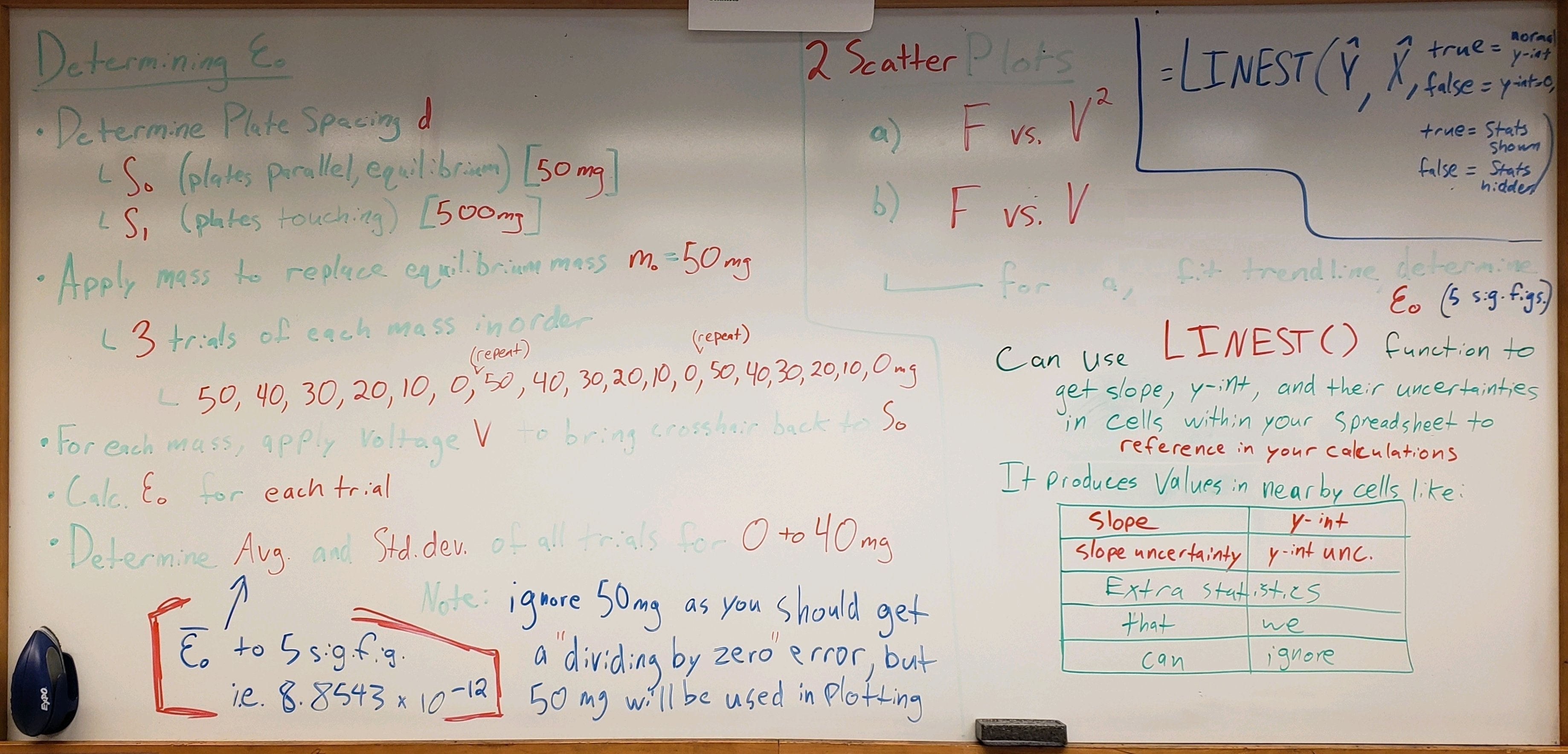
Figure 7:Overview. LINEST() function.
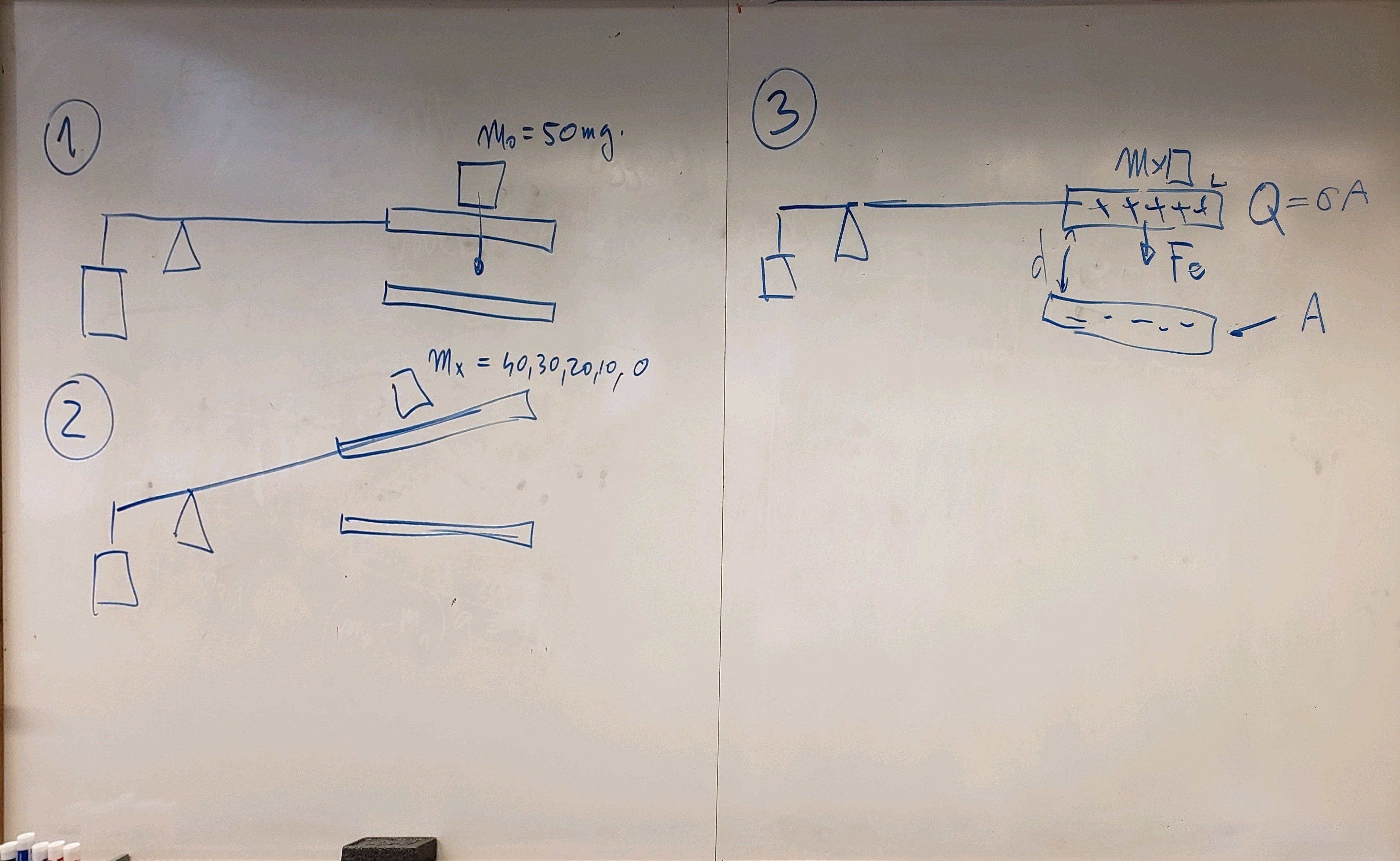
Figure 8:Examples of balancing the plates --- 1) equilibrium (50 mg); 2) less applied mass, not parallel; 3) voltage applied, electric field generated, pulls plates back together to parallel.