Acceleration & Deflection of Electrons
Background
● Background Overview
The instrument used in this experiment is a cathode ray tube [CRT]. When the filament of this device (also called an electron gun) is heated, electrons (mass kg) are freed and given an acceleration. The acceleration is received when the beam of electrons passes through a region of positive potential with respect to the cathode. Consider the schematic of the tube in Figure 1.
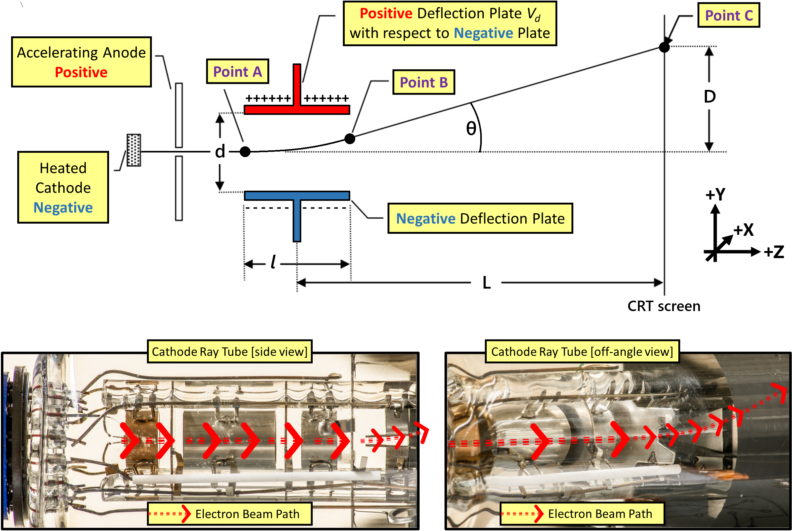
Figure 1:Top) Schematic of the Electron Path in the CRT. Electron enters deflection parallel plates at Point A, exits at Point B, hits screen at Point C having been deflected distance (in the vertical direction for today’s setup). Bottom) Electron beam path through the CRT; after being initially generated by the heater, accelerated toward the screen, brightened by the grid voltage and then focused into a narrow beam, the electrons are deflected up or down as they enter the blackened area of the CRT.
The electrons receive an amount of kinetic energy given by
where is the charge of the electron and accelerating voltage (often just , but changed here to for the sake of consistency with the apparatus used today) is the potential difference between the heated cathode and accelerating anode. Thus the out-of-the-screen velocity in the Z direction (in line towards the phosphor-coated screen of the CRT) is given by
Then, the accelerated electron beam passes between two parallel plates. If a potential is applied between the plates, the electron beam will be deflected toward the positive plate by a force where is the electric field between the plates and is the electric charge. Thus the acceleration in the Y-direction (a.k.a. transverse direction, see Figure 1) due to the deflection voltage is given by
where is the plate separation and is the electron mass. Since the electric field between the plates is approximately uniform, the path of the beam will be parabolic in the region between the plates. This is illustrated from Point A to Point B in Figure 1. The path is a case of an object undergoing uniform acceleration just like an object in projectile motion. After the beam leaves this space, it will continue in a straight line with a out-of-the-screen velocity and a vertical velocity until it strikes the screen at Point C.
The transverse velocity, i.e. in the Y or ‘deflection’ direction we are using today, is given by
where is the time during which the particle is accelerated as it passes through the plates of length . The time t is given by
By combining the above (3), (4), and (5), we obtain the transverse velocity in terms of measurable quantities, namely
Referring to Figure 1, the actual on-screen deflection from the axis is times the time of flight, , over the distance from the end of the deflection plates to the screen. Assuming that , then the time of flight . Since distance equals velocity time, we get
As a result of combining everything we’ve seen so far:
where we see that deflection is directly proportional to deflection voltage . Usually, the geometric quantities are held constant but it is interesting to take a look at the effect of these factors on the deflection.
With longer parallel plates there is more time for the electric field to act on the electron beam and cause deflection. Also, the closer the spacing between the deflection plates , the more intense the field for a given deflection voltage yielding a larger deflection. Finally, the deflection will increase as the accelerating voltage is decreased. This reduces the velocity of the electrons and allows them to spend more time within the deflection field.
The visible spot you see on screen is the result of the energetic electrons releasing their kinetic energy as they impact phosphor atoms. A small portion of that energy is converted to visible light. Most of the energy just heats the screen!
Summing up, the assumptions made in this derivation include:
The geometry of the deflection plates can be considered a ‘parallel-plate’ capacitor configuration. That is, the plates are relatively large and closely spaced. This implies that the electric field is uniform, vertical, and completely contained between the deflection plates.
The distance to the screen is large compared to the horizontal size of the deflection plates ( in Figure 1), so the electron path may be considered to be a straight line from the center of the deflection plate configuration to screen.
The electron beam enters with an initial direction that is parallel to the deflection plates.
● Equipment
Complete Properties of Electrons Apparatus (see Figure 2)
List of experimental cases with their voltages on paper
Cathode Ray Tube (CRT),
19in figure5 mm (major lines) grid pattern on end of CRT (1 mm minor tick marks) (shown later in Figure 3)
Knobs for various electrical control. Note: Voltmeters are for the different sections on the apparatus (See the black-outlined sections on the apparatus for which voltmeters go for which knobs)
1Knobs for controlling X & Y position without changing voltmeter (for calibrating where you place the origin after zeroing the voltmeters with12&13)3Grid, Focus, Accelerating voltage selector (swap between which of17,20,21appears on top voltmeter24)8X & Y-direction deflection voltage selector (swap between which of12,13appears on middle voltmeter23)12X-direction deflection voltage adjustment knob13Y-direction deflection voltage adjustment knob17Grid voltage adjustment knob20Focus voltage adjustment knob21Accleration voltage adjustment knob (acceleration in Z direction)23Voltmeter display for12or13(depending on selection with8)24Voltmeter display for17,20, or21(depending on selection with3)
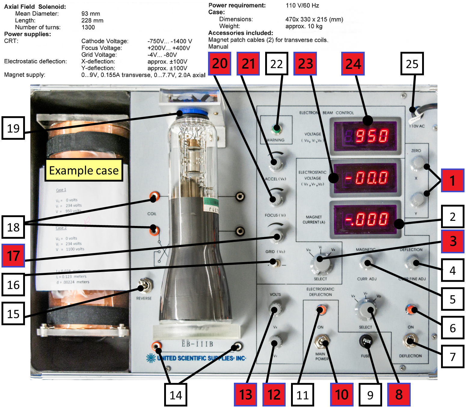
Figure 2:Controls and parameters for the CRT of the Complete Properties of Electrons Apparatus.
Experimental Procedure
● Procedure Preview & Preliminary Setup
All knobs, switches, displays are numbered and will appear as
#in the following steps which correspond to those shown in Figure 2.Turn on the main power switch
10, and wait until the cathode warms up and a bright spot appears on the screen. If it doesn’t appear after ~30 s, an instructor can be of assistance; it’s likely a deflection or zeroing knob pushing the beam off-screen.
● Experimental Data Collection
FOR CASE 1 as listed on apparatus. Set the CRT voltage selector switch
3to read the grid voltage . Adjust the grid voltage to the given value using the grid potentiometer17whose voltage appears on the top voltmeter display24.Now set the CRT voltage selector
3to read the focus voltage . Adjust the focus voltage to the given value using the focus potentiometer20whose voltage also appears on the top voltmeter display24.Next, set the CRT voltage selector
3to read the acceleration or cathode voltage . Set the accel. voltage to the given values using the accel. potentiometer21whose voltage also appears on the top voltmeter display24. ( V, V)Set electrostatic deflection selector switch
8to X-deflection , and set the X-deflection voltage potentiometers13to zero (0.0 V) which appears on the middle voltmeter display23.Set electrostatic deflection selector switch
8to Y-deflection , and set the Y-deflection voltage potentiometers12to zero (0.0 V), again appearing on the middle voltmeter display23.Then, use the ZERO X and Y potentiometers
1to move the bright electron-beam spot to the bottom center of the screen grid (see Figure 3). These knobs do not change the Electrostatic Voltages in23; if the voltages do change, check you are in fact using the ZERO knobs1, not12or13. Make sure to view the CRT head-on so as to account for possible misalignment from the effects of parallax (since the grid is horizontally displaced from the glass of the CRT).
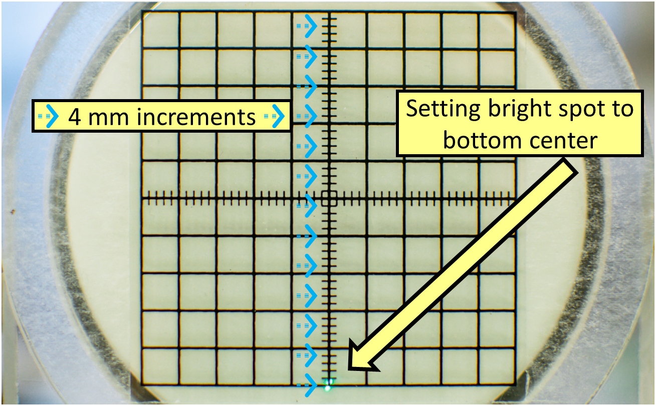
Figure 3:Example of CRT grid and 4 mm spacings.
Ensure the deflection voltage switch
8is set to read the deflection voltage . Since we are only deflecting electrons in the Y-direction, we will refer to the deflection voltage as (i.e. ).Create a common data table, recording the following CRT data and case setups:
= spacing between plates listed on the apparatus
= length of horizontal deflection plates (parallel plates)
= distance from plates to screen of tube
For both cases, record the grid voltages , focus voltages , and accelerating voltages
Create a data table with columns for the deflection voltage and the deflection position (e.g. ). is based on the CRT grid and not to be calculated. At the start of each case, list the acceleration voltage to gelp clarify which case is which.
Record the initial deflection voltage and calculate the ratio of the deflection voltage to the accelerating voltage (). Then record the deflection position on the screen ( at starting point) as well as your best estimate of your uncertainty in deflection position . Then, slowly increase the Y-deflection voltage using the Y-deflection potentiometer
12. Move the bright spot 4 mm in the Y direction; record the deflection voltage , ratio , and . Continue this process every up to for a total of 13 data points. Double check: The acceleration voltage and the horizontal deflection voltage must be constant during this procedure.FOR CASE 2, repeat steps 3 to 12 above using Case 2 data listed on the apparatus including an acceleration voltage of 1100 V.
● Experimental Data Analysis
○ Graphical Analysis --- Deflection Voltage (Plot 1)
Plot both cases on the same graph (we want to see direct comparison):
Your values of deflection distance vs. deflection voltage (i.e. vs. ).
Reminder, is not calculated, but rather just your stated 4 mm increments.
Draw a best fit line through each set of data points and show their equations on the single graph.
For each case, determine the relationship between and . I.e. what is the slope of the best-fit line and the slope’s uncertainty using the
LINEST()function (reminders in Plotting in Excel)? Simplified from (8), we can see in the linear form of :For each case, calculate the expected slope as predicted by the rearrangement of equation (8). Since we don’t know the expected for a given , we can instead use info from (8) to get
For each case individually, determine the RMS in the following to use as an estimate of an overall theoretical position uncertainty from a case’s data set:
a. Use all 13 of your experimental deflection positions and their deflection voltages as well as the slope of your best-fit line found in Step 15 to calculate the square root of the mean of the square difference between your data and the best fit line (i.e. you’re calculating the root mean square or RMS of the difference between what you claim the deflection position is and what the best fit line of your data says the deflection position should be). For each of your 13 data points, you will have a squared difference of .
b. From those 13 values, you can take the mean, then the square root of that mean value for a resulting single value:
where are your claimed 4 mm incremented deflection positions, is your experimental slope, and are your experimentally determined deflection voltages.
○ Acceleration Voltage Analysis
With your CRT still on, change the deflection voltage until the beam is in the upper half of the screen.
Using
3, select , and decrease the acceleration voltage with21as low as it will go. Now, watch the position on the screen as you increase the accelerating voltage to the maximum value. Did the beam go up or down, why?
○ Graphical Analysis --- (Plot 2)
Graphical Analysis, Plot 2: Plot both cases on the same graph (we want to see direct comparison):
Your values of deflection distance vs. deflection voltage to acceleration voltage ratio (i.e. vs. ).
Draw a best fit line through each set of data points and show their equations on the single graph.
For each case, determine the relationship between and . I.e. what is the slope of the best-fit line and the slope’s uncertainty using the
LINEST()function (reminders in Plotting in Excel)? Simplified from (8), we can see (again in the linear form of ):When you are finished with all cases, reset your experimental setup before leaving.
Post-Lab Submission --- Interpretation of Results
● Finalized Spreadsheets
Make sure to submit your finalized data table (Excel sheet).
Please include the relevant plot(s) including (just two for this lab):
vs. with both cases plotted on the same graph.
vs. with both cases plotted on the same graph.
● Post-lab Writeup
In a paragraph, summarize your error analysis. Be both qualitative and quantitative.
What is the precision of your equipment?
What are possible sources of systematic (i.e. affecting accuracy) and random (i.e. affecting precision) errors?
How does the uncertainty (RMS) of your plotted data compare to your estimated position uncertainty on the screen? (i.e. are you over or underestimating single trial uncertainties?)
What are your measured uncertainties, and, based on these uncertainties, how do your final results change? (i.e. do your different measurement and slope uncertainties make your final results larger or smaller?)
If larger or small, are they more or less accurate to expected values?
In a paragraph, summarize the results you have determined, including both analysis methods. Consider:
What was the point of today’s lab; what did we aim to discover?
Do your experimental results (slopes) agree with the expected slopes as predicted by (10)?
Physically, what do your experimental slopes represent?
Does the full data set better represent the physical relationship we’re studying in this lab than your estimation of individual positions (be quantitative)? This is based on your values from the RMS step.
Physically, how is the electron beam deflected in the CRT?
If the accelerating voltage is increased (e.g. Case 1 vs. Case 2), how do you expect the electrons’ beam deflection to change?
I.e. what does the accelerating voltage physically do to the electrons, and how does that effect affect the electrons’ path? Discuss using physical concepts.
For your vs. , how do your lines between the two cases compare (reminder, plotted on the same graph)? (Note: They should overlap somewhat, but why should they overlap?)
The Whiteboard
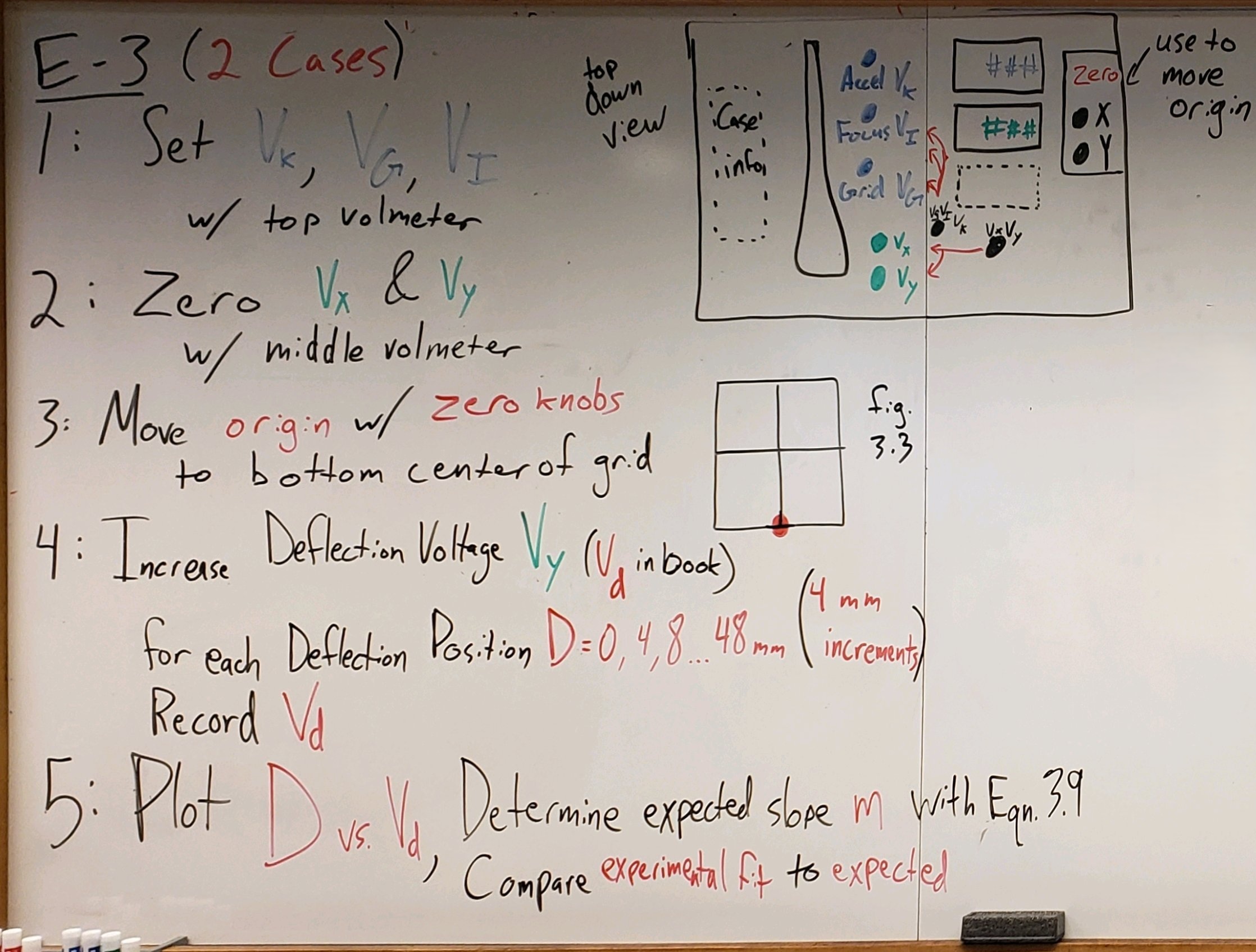
Figure 4:Overview.