|| Example Lab: Simple & Damped Harmonic Motion with Springs & Glider on Level Air Track
Background
● Background Overview
When the magnitude of the net force acting on a body is linearly related to the displacement of the body and is acting in a direction opposite to the displacement, the body will oscillate in simple harmonic motion around the point where the net force is zero. We will investigate the one-dimensional motion of a mass which is constrained by a net force . This linearly related force is said to be obeying Hooke’s Law. That is to say, if the mass is displaced a distance , a restoring force will act in a direction opposite to the displacement with a magnitude equal to the spring constant, , times the magnitude . The independence of the period on the amplitude and the effect of energy loss mechanisms on the motion will also be examined.
Consider the system illustrated in Figure 1. The mass is assumed to be resting on a frictionless surface and is constrained by the two springs shown.
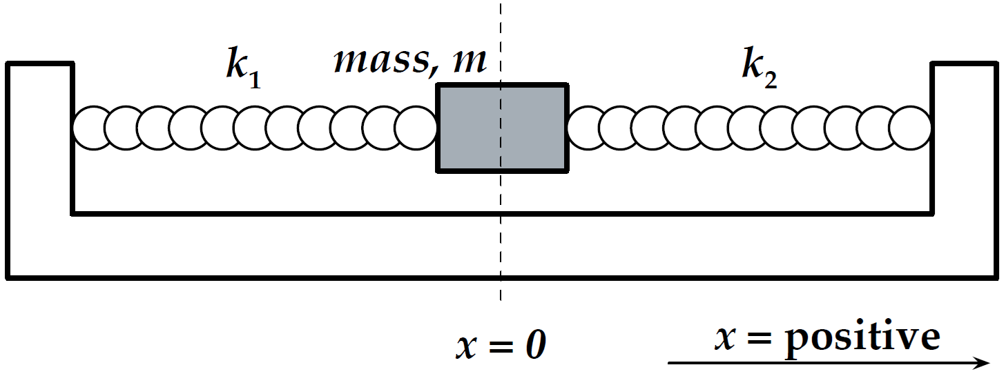
Figure 1:System sketch for Harmonic Motion experiment.
The springs each apply a force according to Hooke’s Law as follows
When , each spring pulls an equal and opposite amount resulting in a net force of at the center equilibrium position.
When the mass is displaced to some point , the net force is given by
These two springs acting together in this manner produce a force , where , or we can say that the force on the mass acts as if one spring was tied to it with an effective spring constant .
If we displace the mass to some position and release it at time , we can determine how the mass will move as a function of time under the influence of the restoring force . Using Newton’s Second Law and the definition of the acceleration , we can write
In order to find a solution to this equation, we need to find a function whose second derivative is the same as the function itself, give or take a constant or two. One such function is
where and are constants. In order to evaluate these constants, we observe what the function must be at known points. One such point is where , that is the release point of the displaced mass. If we substitute the function into (3), we will find that it satisfies the equation if
The quantity is called the angular frequency. From (4), we see that the position of the mass oscillates between the points and as the cosine function oscillates between +1 and -1 as a function of time. The cosine makes one complete oscillation from +1 to -1 to +1 when the quantity goes through radians. The elapsed time for this one complete oscillation is , the period. Thus , or
If the period is the time it takes the mass to make one complete cycle, the frequency will be or . Using (6) we can write the period as
Note that the period of oscillation is independent of the amplitude of the oscillation for this case where there are no energy loss mechanisms.
When the system is started, the mass was displaced a distance and then released. When the system is displaced that distance , a certain energy is given to the system in the form of potential energy stored in the springs in the amount of . Thereafter, this initial energy is the total mechanical energy of the system, and without any energy loss mechanisms, the total energy remains constant. Thus, as the mass moves, it exchanges potential and kinetic energy. If no energy is lost, the mass will always oscillate between the same amplitude and . It will also have the same maximum kinetic energy which occurs at the , or equilibrium position. You can see from (4) and its derivatives, that the displacement, velocity, and acceleration of the mass are related as:
The maximum values of and are dependent on the amplitude . Assume now that there is some energy loss mechanism present as the mass oscillates, e.g.\ some friction on the surface on which the mass is sliding or some air drag on the mass. If energy is lost to such a nonconservative force, then the total energy of the system will decrease. As the total energy decreases, the amplitude, along with the maximum velocity and acceleration will also decrease. Since neither the period nor the frequency of oscillation are functions of the amplitude, they should remain constant. This kind of motion is called damped harmonic motion.
The opposite effect is also true. If a little bit of energy is added during each cycle, then the total energy of the system will increase and be manifested by an increase in amplitude and still no change in period.
Experimental Procedure
● Preview
● Preliminary Setup & Spring Constants
Before assembling the glider and springs on the airtrack, we must determine the spring constants of the two springs. These very light springs are capable of stretching 20 times their rest length. Please be very careful not to damage them through careless handling or overstretching. Create common data table and spring data tables for each of the two springs to measure the spring constant by measuring the extension of the spring at two different displacements from to and .
Create a common data table including:
: Accepted value of acceleration due to gravity for Fairfield University
: masses of large, small, small-with-sail gliders in kg
: uncertainty in masses of large, small, small-with-sail gliders in kg
first spring’s average spring contant and its uncertainty
second spring’s average spring contant and its uncertainty
total effective spring constant and its uncertainty
expected periods and their uncertainties for each of the three glider cases
Measure and record the mass and uncertainty with a triple beam balance for:
large glider
small glider
small glider with sail holder and sail
Create the spring-1 data table for the first spring with a row for each displacement trial including columns of:
height and its uncertainty of the bottom of the loop on the spring (no mass)
applied hanging mass (including hanger) and its uncertainty
gravitational force and its uncertainty due to hanging mass
height and its uncertainty at the bottom of the loop on the spring with the masses
total displacement and its uncertainty due to the applied force
spring constant and its uncertainty
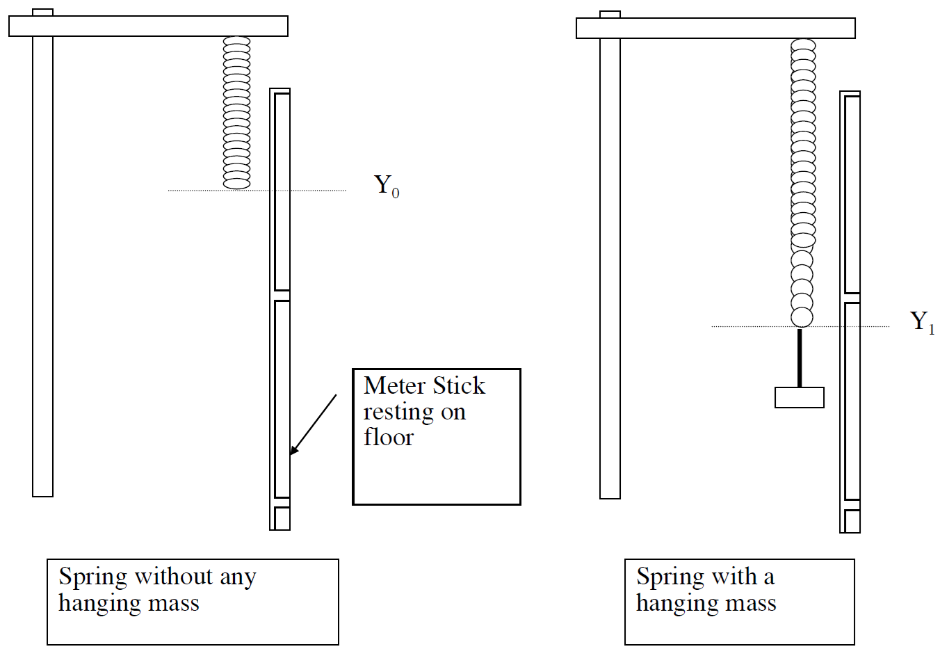
Figure 2:Experimental method to measure for a spring.
For each spring, perform the following steps to determine its average spring constant from two displacement trials. Refer to Figure 2.
Orient the 2-meter stick with the zero end at the top. It is only the change in with force that matters in this measurement.
Attach one end of the spring to the ring stand and allow the spring to hang free with no mass hanging. Record .
Carefully hang enough mass on a weight holder on the end of the spring until it extends a total displacement of from and record the exact position and hangin mass used as (don’t forget the hanger is 50 grams itself). Take the measurements with the spring and any weights hanging stationary.
Calculate the applied gravitational force and total displacement
Calculate the spring constant at this first displacement using (3)
Add a additional mass to the weight holder on the end of the spring until it extends a total displacement of from and record the exact position and mass used as (don’t forget the hanger is 50 grams itself). Take the measurements with the spring and any weights hanging stationary.
Similarly calculate the applied gravitational force and total displacement
Similarly calculate the spring constant at this second displacement using (3)
Repeat the previous steps for the second spring, creating spring-2 data table and determining and for both displacements.
Calculate and record to common data the average spring constants and for each spring.
Calculate and record to common data the effective spring constant that will be acting on the glider.
Calculate the expected periods for each glider from (7).
Once the air supply to the airtrack is on, allow it to flow for several minutes to ensure dust and debris have cleared out.
Level the airtrack. Without the springs attached and the air track resting directly on the tabletop (with the black circle feet), place one of the gliders on the track (somewhere near center) and note any preferential drift of the glider. Adjust the height of the single leg (screw clockwise in to shorted or counter-clockwise out to lengthen) until the air track is level, as indicated by no preferential drift. Check both orientations of the glider on the track to check if the car is asymmetric and has a significant preferential drift on an otherwise level track. If this occurs, make sure to note that for your discussion purposes.
Now that the springs are characterized and air track is level, assemble the larger glider on the track and attach the springs to the glider and the ends of the track as in Figure 1. Again please be careful not to overstretch the springs or allow them to snap back. Keep towards center.
● CASE 1: Large Glider
Create a data table for the measurement of oscillations of the large glider on the air track. You can copy and paste for later cases after you confirm all calculations and methods are accurate. Create enough rows for as many trials --- (e.g. three repetitions (trials) for each of the five initial amplitudes would be 15) including columns for:
Trial number
Lab member’s initials
: Equilibrium position on track scale
: Starting position on track scale at amplitude (that achieves a displacement from equilibrium)
: Starting amplitude (displacement from equilibrium) in meters
Time for ten cycles
: Determined period
Additional rows for mean and standard deviation of the period
To determine the period of oscillation of the mass:
Displace the mass an amplitude of from its equilibrium position, record this position , calculate and confirm the starting amplitude from .
Satisfied with your displacement position, release the glider. When the mass returns to its starting point, start the stopwatch (available at front table) at the zero velocity point (e.g. ). Allow the mass to oscillate through 10 complete cycles and stop the stopwatch at the zero velocity point at the end of the tenth cycle (essentially the same position as the starting point). Record the time for the ten cycles and divide by the number of cycles counted to obtain the period. NOTE: Each group member will measure at the same time to be able to save time while still getting 3 trials per amplitude (if there are groups of two people and you would like additional data, have someone hold two stopwatches to get 3 trials at once).
Use the same glider and repeat for starting amplitudes.
Compare your experimentally determined periods for different starting amplitudes to the large glider’s expected period.
● CASE 2: Small Glider
Reassemble the system with the smaller glider without the sail assembly on the track (Figure 1).
As in ● CASE 1: Large Glider, build a data table and use the same measuring techniques to determine the period for starting amplitudes of Record the time for ten cycles and divide by the number of cycles counted to obtain the period.
Again, compare your experimentally determined periods for different starting amplitudes to the small glider’s expected period.
● CASE 3: Small Glider with Sail
The third experiment in this lab focuses on measuring the damped oscillation of the small glider WITH A SAIL. Instead of starting at different amplitudes, you will start from the same starting amplitude . You will count across a range of oscillations, from 5 up to 30 oscillations, to determine how much the final amplitude changes over time.
Create a data table for the measurement of oscillations of the small glider with a sail on the air track. There will be 6 trials, one for each range of oscillations . Create enough rows for as many trials including:
: number of cycles
: equilibrium position
: starting position
: starting amplitude
: final position after cycles
: final amplitude (final position minus equilibrium position)
the total time
the average period
Place the paper sail assembly on the small glider. Only 1 trial needed per number of cycles.
Use a single starting amplitude of from the equilibrium position. Record both the equilibrium position and your starting position; determine and record the amplitude from (should be Each of the following steps will be started from this same starting position and amplitude.
Displace the glider with its sail to the starting position and release it.
When the mass returns to its starting point, start the stopwatch at the zero velocity point (e.g. ).
At the end of the fifth cycle, stop the stopwatch and capture the glider by gently pressing your finger on the edge of the glider as gets to its maximum amplitude point, i.e. when . Note: Be sure to use the same point on the glider that you used to determine the equilibrium point and the starting point.
Record the final position and calculate the final amplitude .
Record the total time for the current trial, divide by the measured to obtain the average period.
Compare this with the expected period from (7), remembering the total mass of the glider plus sail assembly.
Repeat previous steps five more times, each time starting the glider from the same starting amplitude, and allow the glider to oscillate five additional cycles more than the previous measurement. Only 1 trial needed per number of cycles.
● Graphical Analysis
For Case 1 and 2, plot the period (-axis) vs. the starting amplitude (-axis). Include trendline.
For Case 3
Plot the period (-axis) vs. the final amplitude (-axis). Include trendline.
Plot the final amplitude vs. .
● Summary & Cleanup
Create a summary table of your data (e.g. relevant final result values, averages, and differences from each case).
When you are finished, reset your experimental setup before leaving.
Post-Lab Submission — Interpretation of Results
● Finalized Spreadsheets
Make sure to submit your finalized data table (Excel sheet).
Please include relevant plot(s) including:
Cases 1 & 2:
vs.
Case 3:
vs.
vs.
● Post-lab Writeup
In a paragraph, summarize your error analysis. Be both qualitative and quantitative.
What is the precision of your equipment?
What are possible sources of systematic (i.e. affecting accuracy) and random (i.e. affecting variance) errors?
Discuss those from spring characterization
Discuss those in the undamped cases
Discuss those in the damped case
How do your measured uncertainties in hanging mass and spring constants affect your expected periods; by how much; which showed a larger impact?
In a paragraph, summarize the results you have determined in each case. Consider:
For all three cases, how do the the measured periods of the glider compare to expected periods? I.e. do they agree within uncertainty and standard deviation ranges?
Comment (qualitatively) on the behavior of the curves from each plot. Do the trends make sense? Explain with physical concepts.
From the damped-oscillator plot, what do you expect amplitude of the glider to be after 50 cycles?
Does the amplitude affect the period? Why or why not? Argue a physical answer supported by your data; discuss whether your data supports the theory for:
An undamped oscillator
An damped oscillator
How does the period depend on the mass of the glider? Is this expected?
How does an increased air drag affect the result for the period?
How does the amplitude depend on the number of cycles (relate this to energy conservation)?
The Whiteboard
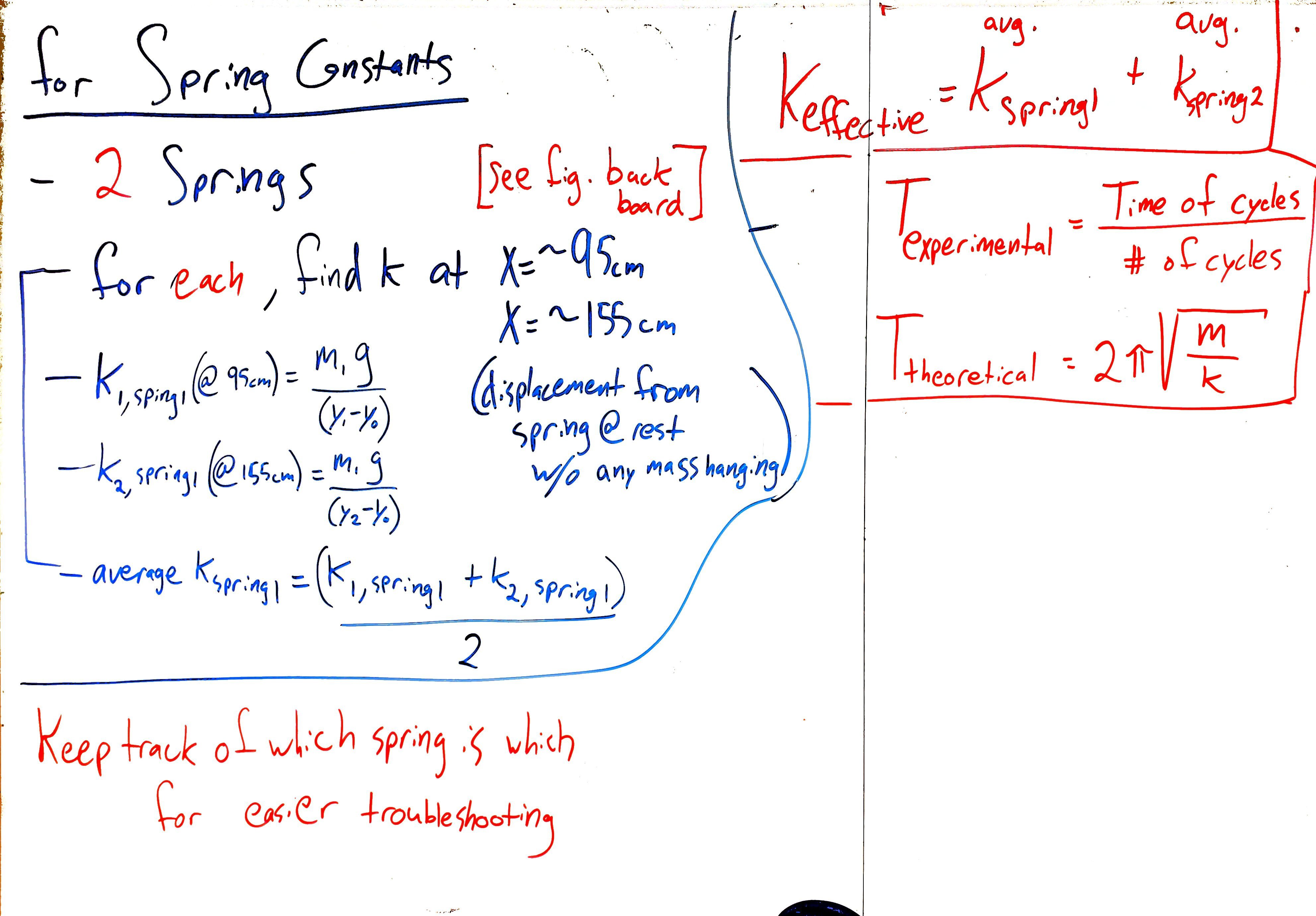
Figure 3:Overview for spring constants.
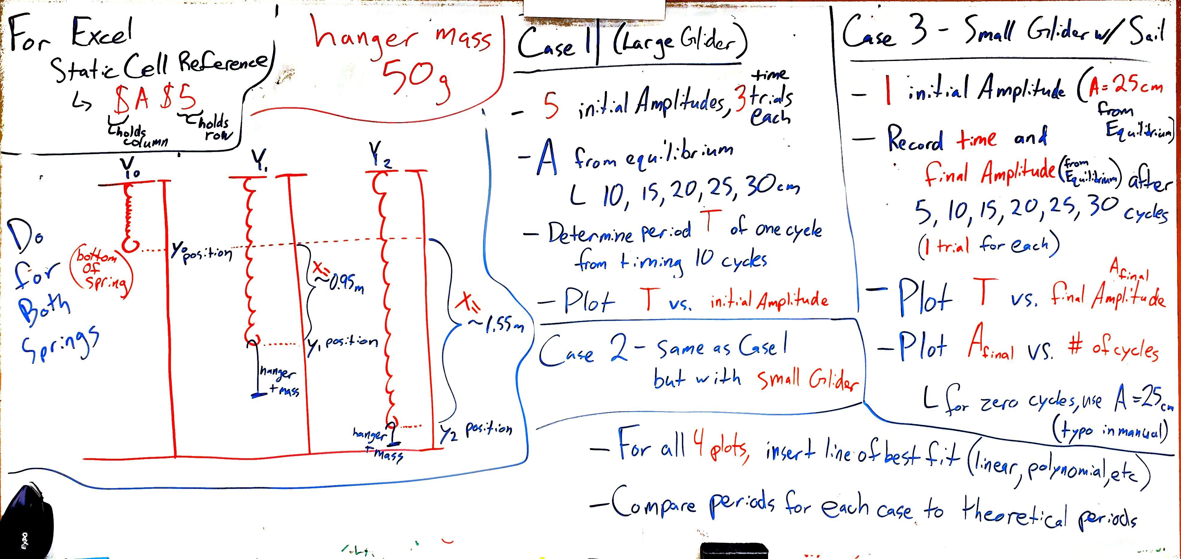
Figure 4:Overview for oscillations of simple harmonic motion and damped harmonic motion.
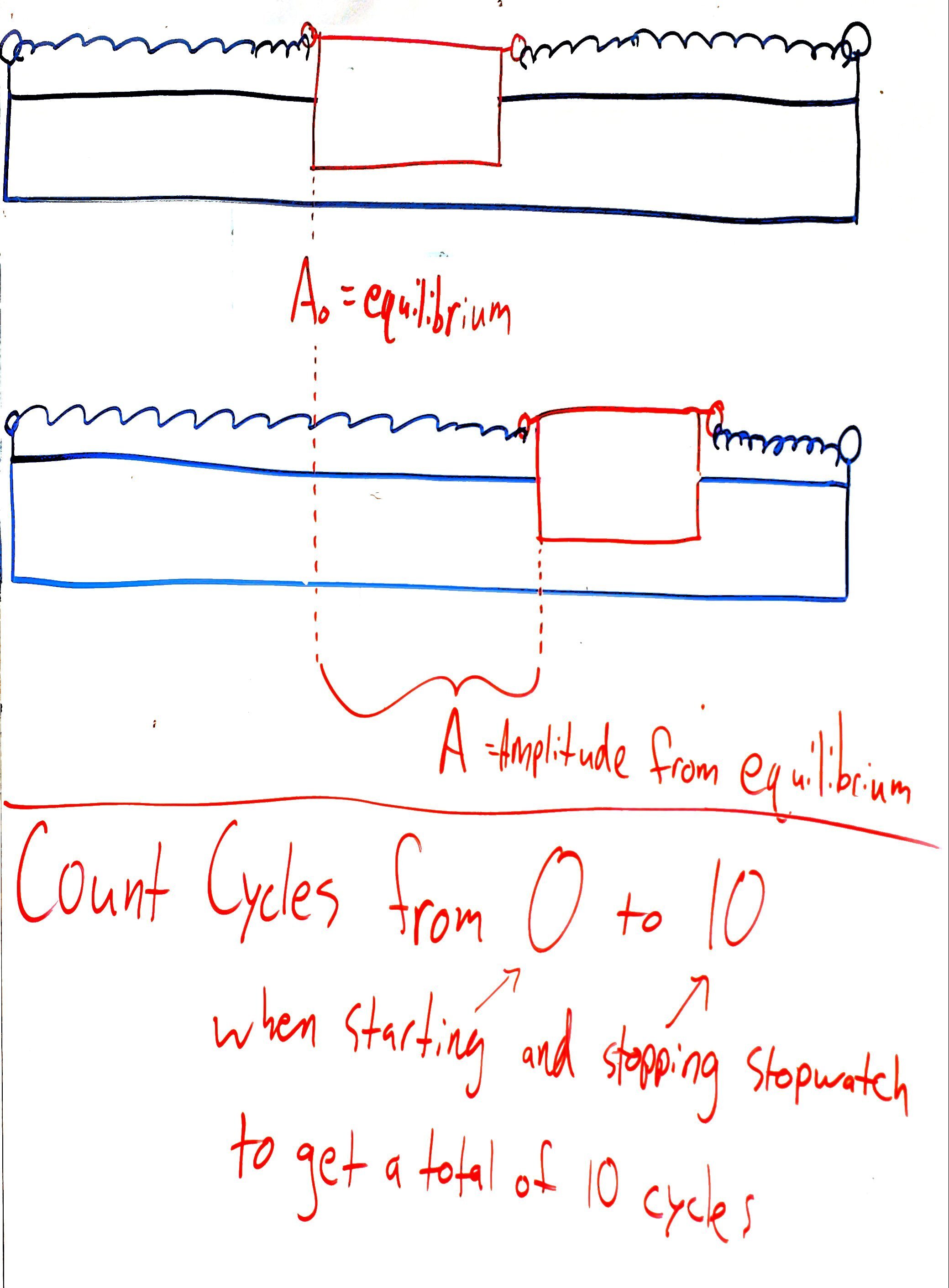
Figure 5:Amplitude measured from equilibrium in image, position used in procedure. Cycle counting suggestions.